Table of Contents

This is the first in a series of three posts detailing the Hilbert Sort problem, its solution, and its implementation. This post sets up the problem.

• Hilbert Sort: Motivation
• Hilbert, Peano, and Space-Filling Curves
• Constructing a Hilbert Curve
• Performing a Hilbert Sort
• Problem Statement
• References

Hilbert Sort: Motivation

In the next few series of posts, we will cover the Hilbert Sort problem, how it works, and how to implement it.
However, before we describe the problem further, let's start with some motivation for solving this problem.

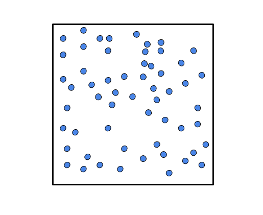
Suppose we're dealing with a very large number of independent objects on a 2D coordinate grid, each with a coordinate location \((x,y)\). (For example, a large population of particles moving in a fluid, or a large number of characters on a map in a game.)

Here is our box of particles:

Now, suppose that we have more data than can be handled by a single computer, and we want to arrange the data on different computers. However, we want to arrange the data in such a way that we preserve the spatial characteristics of the data.

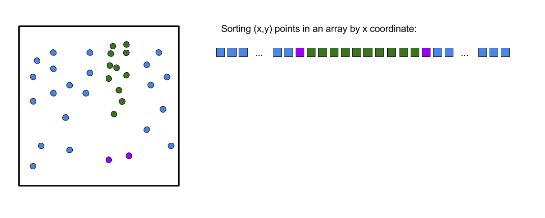
If we implement a naive sort method for Cartesian points that sorts points by x coordinate value, breaking ties with the y coordinate value, we end up with points that are neighbors in space, but far away in the data container's storage (like an array). This is particularly true if there are large crowds of points in the grid.

Here is an illustration of a set of points and their resulting storage schema in an array that sorts points by x coordinate. It shows two purple particles, close by in space, but with
several green particles further away distance-wise but not with respect to the x coordinate. The spatial locality of points is not preserved in the data container, so clearly, a better method of sorting and organizing points is needed.

An alternative to this schema that yields better locality properties, but that leads to a much higher cost for sorting points, involves iterating over each point, and for each point, finding the closest points to it in space. However, this itself requires iterating over each point. This approach ends up walking over each point (the point whose nearest neighbors we are finding), and doing a second nested walk over each point (checking if a point is a nearest neighbor to this one). The overall cost of doing this is \(O(N^2)\).

It is a deceptively tricky problem: how to organize a large group of points in a way that preserves spatial locality?

But first, we'll cover the topic of space filling curves, then return to this topic.

Space Filling Curves

Mathematician Giuseppe Peano was a prolific teacher and researcher known for many things, but one of his more curious ideas is known as the Peano Curve. Peano was attempting to answer the question of whether a continuous curve could be bounded by a finite space, and he invented a counter-example: a recipe for breaking a curve into parts that can be replicated and repeated and applied to the copies as many times as desired, and always result in a continuous curve.

The way that space-filling curves in general are constructed is to create a pattern, then scale it down and repeat it, attaching subsequent scaled-down, repeated curves. Peano simply invented the first curve; there are many variations on the original space-filling curve idea (including the Hilbert Curve - more on that in a moment).

The original 1890 paper by Giuseppe Peano is entitled "Sur une courbe, qui remplit toute une aire plane", published in 1890 in Mathematische Annalen I, Issue 36. Unfortunately, it has no pictures, but here is a rendering from Wikimedia Commons:

(Link to original on Mediawiki Commons)

Now, the Peano curve was nice, but it had some mathematical properties that made it difficult to deal with. So in 1890, David Hilbert published a follow-up paper in Mathematische Annalen I Issue 38, entitled "Ueber die stetige Abbildung einer Linie auf ein Flächenstück", which slightly modified the recipe to create a curve with more elegant mathematical properties.

Also, he included pictures.

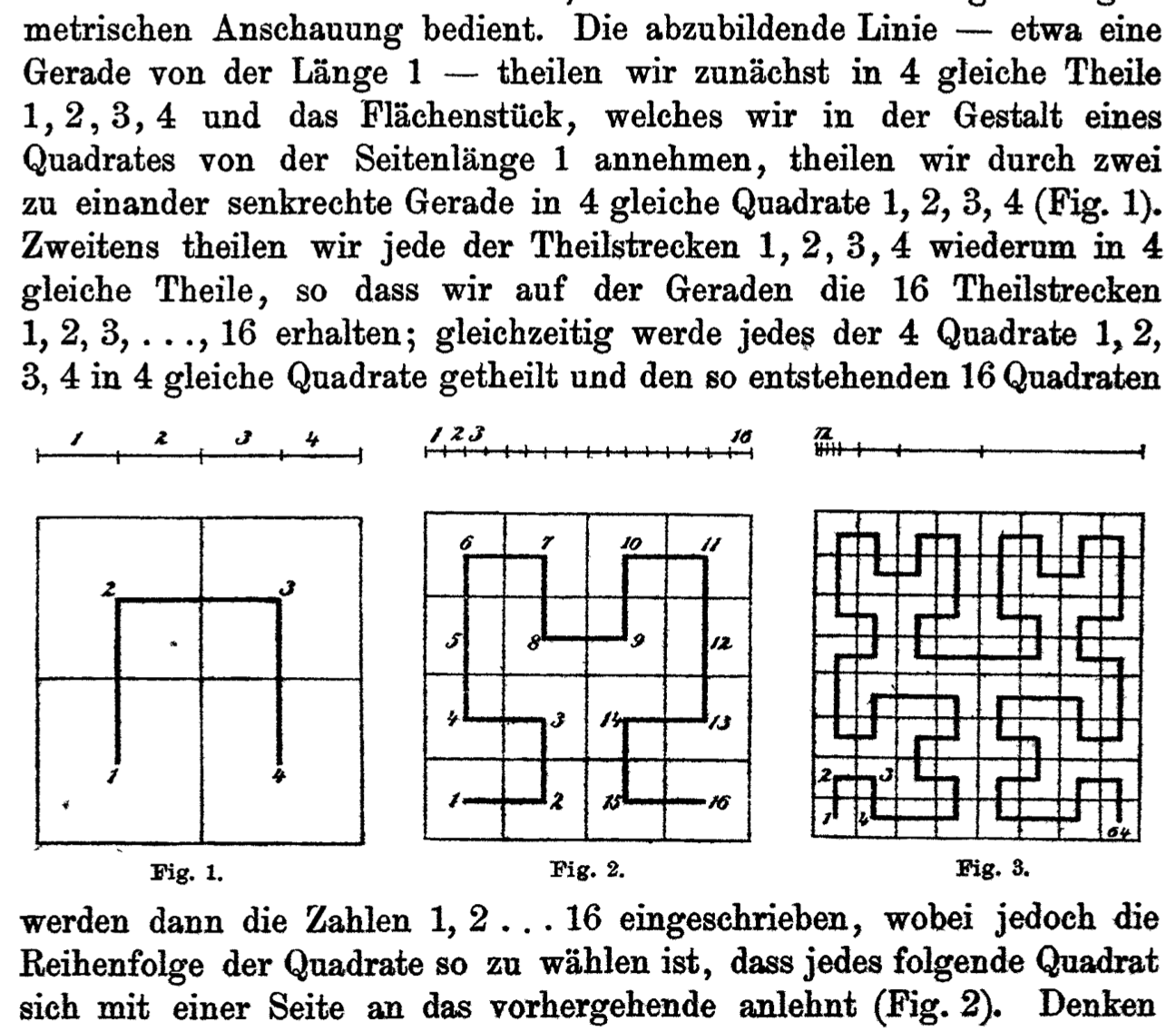
Here is the first set of figures from Hilbert's original 1890 paper:

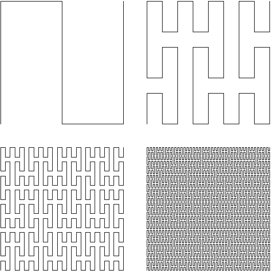
And here is a slightly cleaner rendering of the Hilbert Curve pattern repeated six times:

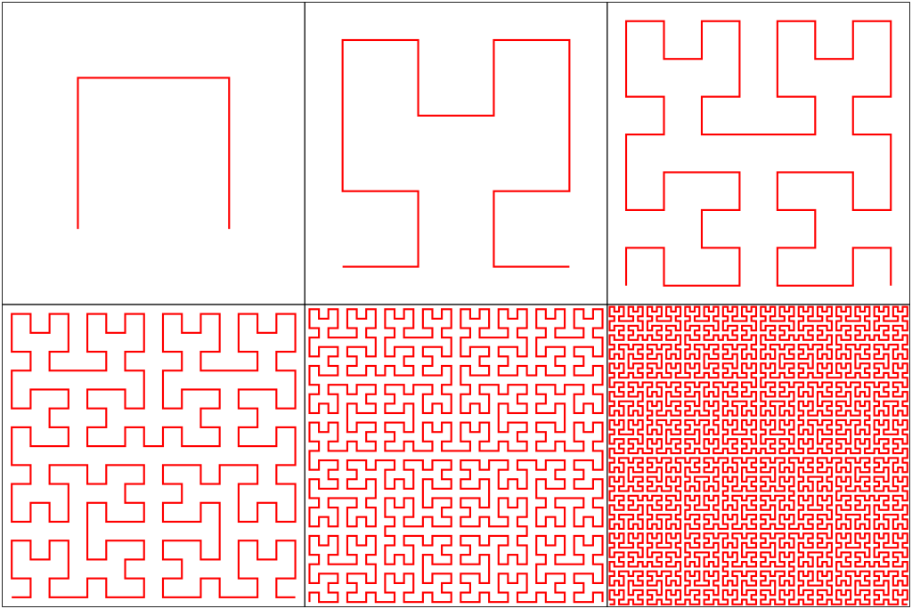
(Link to original on Wikimedia Commons)

From the abstract of Hilbert's paper:

Peano has recently shown in the Mathematical Annals, 2 by an arithmetical observation, how the points of a line can be mapped continuously to the points of a surface part. The functions required for such a mapping can be produced more clearly by using the following geometrical view. Let us divide the line to be represented-about a straight line of the length 1-into four equal parts 1, 2, 3, 4, and the surface which we assume in the form of a square of the side length 1 Straight into 4 equal squares 1, 2, 3, 4 (Fig. 1). Secondly, we divide each of the partial sections 1, 2, 3, 4 again into 4 equal parts so that we obtain on the straight the 16 partial sections 1, 2, 3, ..., 16; At the same time, each of the 4 squares 1, 2, 3, 4 is divided into 4 equal squares, and the numbers 1, 2, ..., 16 are then written to the resulting 16 squares, That each successive square follows the previous one with one side (Fig. 2). If we think of this method, as shown in Fig. 3, the next step, it is easy to see how to assign a single definite point of the square to any given point of the line. It is only necessary to determine the partial stretches of the line to which the given point falls. The squares indicated by the same numbers are necessarily in one another and include a certain point of the surface piece in the boundary. This is the point assigned to the given point. The image thus found is unambiguous and continuous, and vice versa, each point of the square corresponds to one, two, or four points of the line. Moreover, it appears remarkable that, by a suitable modification of the partial lines in the squares, a clear and continuous representation can easily be found, the reversal of which is nowhere more than three-fold.
- David Hilbert, "Über die stetige Abbildung einer Linie auf ein Flächenstück", Mathematische Annalen Vol 38

Thanks to Google Translate for an incredible job.

Constructing a Hilbert Curve

To construct a Hilbert curve, you just have to follow the recipe. It doesn't matter what your square contains so far, or how many levels in you are, whether it's the first curve or the five hundredth:

1. First, take yer square.

2. Second, quadruple yer square. That means, make four copies, that all make a square.

3. Now rotate the bottom left and bottom right via diagonal reflection.

4. Fourth step is, you're done - that's you're new square!

Performing a Hilbert Sort

We will omit a proof of the statement, but given a set of unique (x,y) points, we can always construct a minimal-size Hilbert Curve that visits each point only once.

Points can be sorted, then, according to when they would be visited by said Hilbert Curve. And this ordering provides better preservation of spatial locality and structure of points when aligning them in memory, because these space-filling curves are recursive and preserve spatial locality in a top-down fashion.

For example, if we have two points in our square, one in the lower left and one in the lower right, and we are sorting them via a Hilbert Sort, we definitely know that a Hilbert curve constructed to visit both of these points will definitely visit the lower left point (the quadrant where the Hilbert curve starts) before it visits the lower right point (in the quadrant where the Hilbert curve stops).

This requires thinking about \((x,y)\) points in the box in terms of quadrants, and the order in which the Hilbert curve will visit each quadrant or region, rather than thinking in terms of the explicit Hilbert curve that will visit each particular \((x,y)\) point:

This is a subtle shift in the thinking about this problem, but it is crucial to a successful implementation of a Hilbert sort. The problem that will follow, which asks to implement the Hilbert sort, has many distracting details, including the Hilbert curve itself.

Remember, in Hilbert sort, the end goal is not the curve itself, but the sort order.

Here is how the quadrant-by-quadrant partitioning to sort elements ends up looking when applied repeatedly:

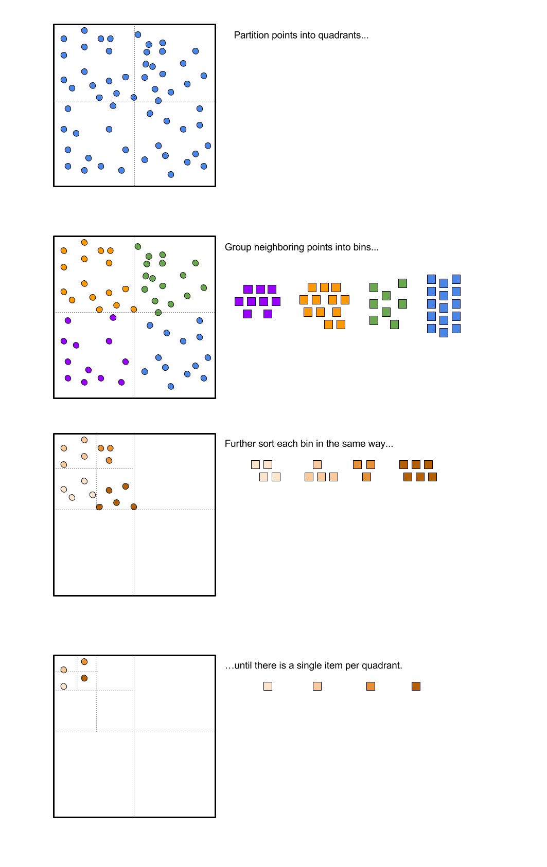
It is important to note that the two diagonal reflections happening in the corners are the trickiest part of this problem. We will cover this operation in greater detail in the solution blog post.

Problem Statement

Following is a paraphrased problem statement from the original ACM ICPC Regional Programming Competition problem statement that this problem and its solution was based on.

"If points \((x,y)\) are sorted primarily by x, breaking ties by y, then points that are adjacent in memory will have similar x coordinates but not necessarily similar y, potentially placing them far apart on the grid. To better preserve distances, we may sort the data along a continuous space-filling curve.

"We consider one such space-filling curve called the Hilbert curve...

"Given some locations of interest, you are asked to sort them according to when the Hilbert curve visits them. Note that while the curve intersects itself at infinitely many places, e.g., at \((\frac{S}{2}, \frac{S}{2})\), making S odd guarantees all integer points are visited just once."

Here is an example input file, giving a set of points on an \(M \times N\) grid:

    14 25
    5 5 Honolulu
    5 10 PugetSound
    5 20 Victoria
    10 5 Berkeley
    10 10 Portland
    10 15 Seattle
    10 20 Vancouver
    15 5 LasVegas
    15 10 Sacramento
    15 15 Kelowna
    15 20 PrinceGeorge
    20 5 Phoenix
    20 10 SaltLakeCity
    20 20 Calgary

The corresponding output can be verified intuitively, assuming the coordinates given above are accurate! Here is the output. Indeed, the order in which each city is visited is what we would expect if we drew a space-filling Hilbert curve over a map of the western United States and Canada.

    Honolulu
    Berkeley
    Portland
    PugetSound
    Victoria
    Vancouver
    Seattle
    Kelowna
    PrinceGeorge
    Calgary
    SaltLakeCity
    Sacramento
    LasVegas
    Phoenix

Now that we've used up all of our space here describing the problem, in a follow-up post we will go into greater detail about how to solve the problem conceptually, and come up with some pseudocode for a recursive method (since this is a recursive task). Then, a third post will go into greater detail about the final Java code to perform this task.

References

1. "ACM Pacific Region Programming Competition." Association of Computing Machinery. Accessed 19 June 2017. <http://acmicpc-pacnw.org/>

2. "Sur une courbe, qui remplit toute une aire plane." G. Peano. Mathematische Annalen 36 (1890), 157–160. (pdf)

3. "Über die stetige Abbildung einer Linie auf ein Flächenstück." D. Hilbert. Mathematische Annalen 38 (1891), 459–460. (pdf)

4. "Hilbert Curve." Wikipedia: The Free Encyclopedia. Wikimedia Foundation. Edited 29 April 2017. Accessed 23 June 2017. <https://en.wikipedia.org/wiki/Hilbert_curve>

5. "Peano Curve." Wikipedia: The Free Encyclopedia. Wikimedia Foundation. Edited 16 October 2016. Accessed 23 June 2017. <https://en.wikipedia.org/wiki/Peano_curve>