This is the second in a series of three posts detailing the Hilbert Sort problem, its solution, and its implementation. This post solves the problem.

Hilbert Sort Problem

In the prior post, we covered the Hilbert Sort problem, but we state it once more succinctly here before detailing a solution to the problem.

The Hilbert Sort problem asks the following: given a set of labeled $(x,y)$ points, how can we sort the points according to the order in which they are visited by a space-filling Hilbert curve?

Revisiting the example input and output provided, the input provides the number of points and size of the grid on the first line, followed by each point's coordinates and label.

Input:
    14 25
    5 5 Honolulu
    5 10 PugetSound
    5 20 Victoria
    10 5 Berkeley
    10 10 Portland
    10 15 Seattle
    10 20 Vancouver
    15 5 LasVegas
    15 10 Sacramento
    15 15 Kelowna
    15 20 PrinceGeorge
    20 5 Phoenix
    20 10 SaltLakeCity
    20 20 Calgary

Output:
    Honolulu
    Berkeley
    Portland
    PugetSound
    Victoria
    Vancouver
    Seattle
    Kelowna
    PrinceGeorge
    Calgary
    SaltLakeCity
    Sacramento
    LasVegas
    Phoenix

Space is the Place

To solve the Hilbert Sort problem, we have to avoid the temptation to think about the Hilbert curve and the way that it is constructed. While we spent quite a bit of time talking about the Hilbert curve and how it is constructed, the curve itself is not what we are interested in - we are interested in the order in which the points are visited.

Also remember, the motivation of solving the Hilbert Sort problem is to arrange spatial $(x,y)$ points so closer points are nearer together.

No matter how many iterations of the Hilbert curve we end up drawing, we always apply the same procedure: cut the square into four quadrants, reflect the southwest corner about the bottom left to top right diagonal, and reflect the southeast corner about the bottom right to top left diagonal.

We will always visit points in the southwest quadrant before we visit points in the northwest quadrant; we will always visit points in the northwest corner before we visit points in the northeast corner; etc.

The Reflections

The trickiest part of the Hilbert Sort problem is the reflection that happens to the lower left and lower right quadrants.

Reflected Quadrants

Start with the first step of the Hilbert sort - take a square with points contained in it. Split the square into four quadrants (with the intention of creating four sub-problems). However, to conform to the Hilbert Curve construction process, the lower left and lower right squares must be reflected. The lower left square is reflected about the bottom left to upper right diagonal, while the lower right square is reflected about the bottom right to upper left diagonal.

Convince yourself of this by studying the curve construction procedure as illustrated by Hilbert himself in his 1890 paper (a.k.a., Hilbert Illustrates A Hilbert Curve):

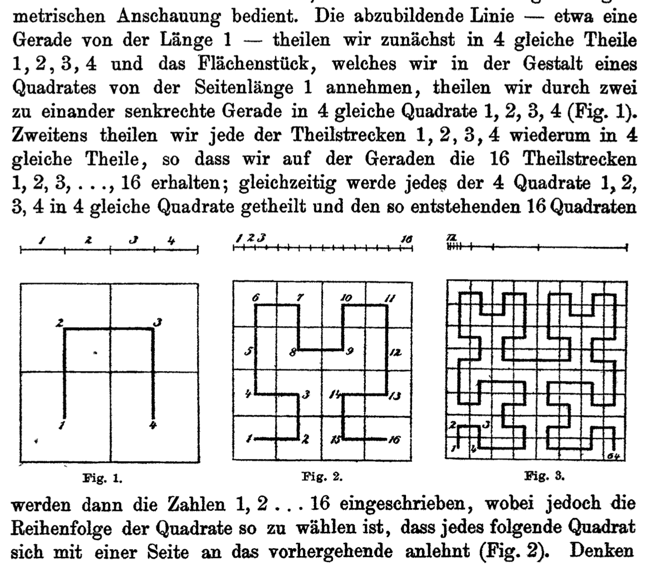
Hilbert Illustrates Construction of Hilbert Curve

We are working toward a recursive method - and recursive methods call themselves repeatedly, apply to subproblems that are trivially similar. However, to translate this into a recursive problem, we have to deal with the rotations within the current recursive step, in such a way that we don't need to know the orientation of the prior square to know the order in which to visit the squares - it is always southwest, northwest, notheast, southwest.

After we split the squares into quadrants, after we toss out any quadrants with no points, we walk through each of the four quadrants in order (southwest, northwest, northeast, southwest). If there is a single point in the quadrant, we add it to the priority queue.

It is here that we take care of the rotation - before we recursively call the Hilbert sort method on the quadrant itself.

Scaling

We have a prescribed order for the four quadrants in the current recursive level, and the current recursive level is working its way through each of those four quadrants. But remember, our algorithm only cares about the order of points. It does not care about the $(x,y)$ location. So we can ireflect $(x,y)$ points by changing their $(x,y)$ coordinate locations. Ultimately we are only changing the program's internal representation of each point, not the original data on disk, so we can think of $(x,y)$ as mutable for our purposes.

This is an important part of our solution: scaling (and reflecting) each quadrant before recursively calling the Hilbert sort method on the points contained in it.

If we are considering a single quadrant of dimensions $\frac{S}{2} \times \frac{S}{2}$, containing points $(x,y)$, we may be able to pass in the corners of our square, plus the $(x,y)$ points contained in it. However, as our squares get smaller, the distance between points gets smaller as well, so this has an upper limit as to how many points it can sort.

On the other hand, we can avoid passing all that information around and using doubles, by just rescaling everything to the given quadrant. We want each recursive level to completely forget about where in the recursive stack it is, how large its square is relative to the original, etc. All it should be doing is solving the same problem repeatedly - which is what recursion is best at. If we double the sides of the square, we get a shape with original size $S \times S$. To keep the points shifted correctly we double their $(x,y)$ coordinates to $(2x, 2y)$.

Once this transformation is performed, we are ready to call the Hilbert Sort function recursively - for the northwest and northeast quadrants only. The southwest and southeast quadrants still have a ways to go.

Reflection

In addition to the scale-up transformation, southwest and southeast qaudrant points must be reflected about their diagonals.

Here's an example of what the process looks like in action:

Hilbert Sort Poster Flowchart

Solving the Reflection Problem

The above section described where in the process the reflection of the $(x,y)$ points should happen. The process of applying the reflection differs between the southwest and southeast quadrants.

In the southwest quadrant, points are being reflected about the diagonal line $y=x$, so the reflection of $(x,y)$ points in the southwest quadrant can be performed by swapping the $x$ and $y$ values of all of the points in that quadrant.

In the southeast quadrant, the points are refelected about the diagonal $y = -x$, but it is not quite $y = -x$, given that there is an offset of a half-quadrant width on the left.

After an $(x,y)$ point is transformed, it has a height equal to the distance from the point's x coordinate to the start of the qudarant. In equations,

$$ y = S - x $$

Further, after an $(x,y)$ point is transformed, the distance from the top of the bounding box to the former y coordinate is the new x coordinate,

$$ x = \frac{S}{2} - y $$

The relative x coordinates of each point (relative meaning, 0 starts at the beginning of the curent square, rather than the whole square) are the x coordinates minus the half-quadrant width.

Once these reflections are performed, we pass the resulting $(x,y)$ points on to a new Hilbert sort. The new Hilbert sort will be operating on an $S x S$ square, as before. Importantly, the $(x,y)$ points have been transformed in such a way that the order in which the Hilbert curve visits each point has not been affected.

Hilbert Sort Procedure

The implementation strategy is, obviously, recursive. What we want to do at each level is: * Start with a square and points contained in the square. * Cut the square under consideration into four quadrants. * Apply a transformation to each square so that it is re-oriented in a manner that matches our original Hilbert curve.

Once each of those squares goes through all of its respective recursive calls, it will return a sorted list of points. Then we will know what to do - we collect each of the sorted points from each of the four quadrants in order, maintain that order, and return those sorted quadrants.

To nail down the details, treat the square under consideration as ranging from $(0,0)$ to $(S,S)$.

Each time we cut a square into quadrants, we re-orient ourselves as to where $(0,0)$ is located and which quadrants will be visited in which order. If we are in the lower left quadrant, $x$ is below $\frac{S}{2}$ and $y$ is below $\frac{S}{2}$, so we rotate and reflect by swapping x and y:

        X -> Y
        Y -> X

If we are in the upper left quadrant, x is below $\frac{S}{2}$, y is above $\frac{S}{2}$, so subtract $\frac{S}{2}$ from y and we're done.

        X -> X
        Y -> Y-(S/2)

If we are in the upper right quadrant, x is above $\frac{S}{2}$, y is above $\frac{S}{2}$, so subtract $\frac{S}{2}$ from both

        X -> X - S/2
        Y -> Y - S/2

If we are in the lower right quadrant, our x and y values are now relative to the quadrant bounding box. The distance to the top of the bounding box to the y coordinate becomes our new x coordinate, while the distance from the right of the bounding box S to the x coordinate becomes our new y coordinate:

        X -> S/2 - Y
        Y -> S - X

Recursion always requires a base case and a recursive case. Our "base case" is the simple comparison of one or no points in each of our four quadrants. If we get to this base case, we know the order in which the Hilbert Curve will visit each of those points.

If we are not at the base case, if we have a large number of points to sort, we can bin together all the points in a given quadrant, and consider the order in which those points go with an additional level of finer granularity.

Pseudocode

set square dimension S

create unsorted queue
load points into unsorted queue

create sorted queue
sorted queue = hilbert_sort( unsorted queue, square dimension )

Now here is the Hilbert sort function:

define hilbert_sort( unsorted queue, square dimension ):
    create southwest queue
    create northwest queue
    create northeast queue
    create southeast queue
    for each point:
        if in southwest:
            create new point using X -> Y, Y -> X
            add to southwest queue
        if in northwest:
            create new point using X -> 2X, Y -> 2Y - S
            add to northwest queue
        if in northeast:
            create new point using X -> 2X - S, Y -> 2Y - S
            add to northeast queue
        if in southeast:
            create new point using X -> S - 2Y, Y -> 2S - 2X
            add to southeast queue

        hilbertsort(southwest queue, square dimension)
        hilbertsort(northwest queue, square dimension)
        hilbertsort(northeast queue, square dimension)
        hilbertsort(southeast queue, square dimension)

        create new results queue
        add points from southwest into results queue
        add points from northwest into results queue
        add points from northeast into results queue
        add points from southeast into results queue
        return results queue

References

"ACM Pacific Region Programming Competition." Association of Computing Machinery. Accessed 19 June 2017. <http://acmicpc-pacnw.org/>
"Über die stetige Abbildung einer Linie auf ein Flächenstück." D. Hilbert. Mathematische Annalen 38 (1891), 459–460. (pdf)
"Hilbert Curve." Wikipedia: The Free Encyclopedia. Wikimedia Foundation. Edited 29 April 2017. Accessed 23 June 2017. <https://en.wikipedia.org/wiki/Hilbert_curve>

CSE 143 Final Project: Hilbert Sort: 2. The Solution Algorithm

Table of Contents