- Intro
- The Graphs We Are Solving
- Guava TSP Solution
- Improving the Guava TSP Solution
- Timing Results
- Future Work
Intro
In a prior blog post we introduced you to the traveling salesperson problem (TSP), which involves finding the shortest path through every city in a group of cities connected by a network of roads. Using Google Guava, we have implemented a solution to the TSP in Java.
Our philosophy toward timing, profiling, and optimization is that it is always best to work from data - and timing is the first place to begin collecting data. As we will show in this blog post, simply timing your function for different problem sizes can reveal scaling behavior that indicates bottlenecks, bugs, or inefficiencies in the algorithm.
In this post, we use simple timing tools and a spreadsheet to plot scaling behavior and identify bottlenecks in the traveling salesperson problem code. Fixing the bottleneck led to a reduction in cost of two orders of magnitude.
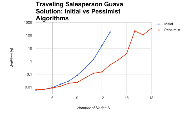
Here's a preview:
In this post we'll cover what we did to time the problem, the initial results, and the algorithm improvement that led to the massive performance improvement.
But first, let's look at some of the graphs that are being solved.
The Graphs We Are Solving
Let's start by having a look at some of the graphs we will be solving, and the representation of the problem.
Visualizations of Graphs
The first few graphs start out simple: here is a randomly generated 4-node traveling salesman problem (we wil cover the code that generates the graph pictured here in a moment):
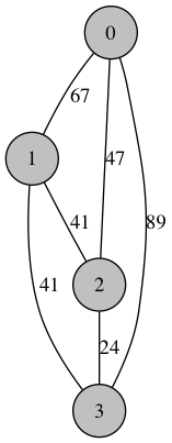
Shortest Route: [0, 2, 3, 1] Distance: 112.0
Here is another randomly generated graph with 5 nodes:
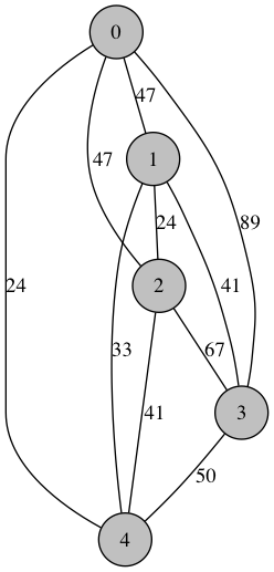
Shortest Route: [0, 4, 2, 1, 3] Distance: 130.0
With 6 nodes:
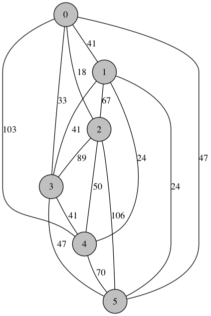
Shortest Route: [0, 2, 4, 1, 5, 3] Distance: 163.0
But problem of this sise are still trivially easy for a processor to handle. Our inefficient, first-pass algorithm started to show signs of eating up CPU cycles at around 9 nodes (albeit less than 1 second). Here is the graph with 9 nodes:
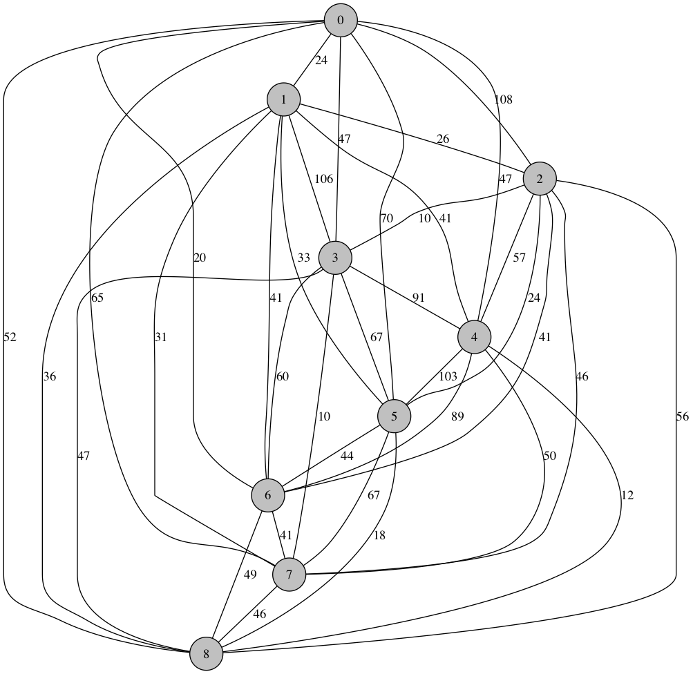
Shortest Route: [0, 6, 1, 7, 3, 2, 5, 8, 4] Distance: 166.0
With 12 nodes:
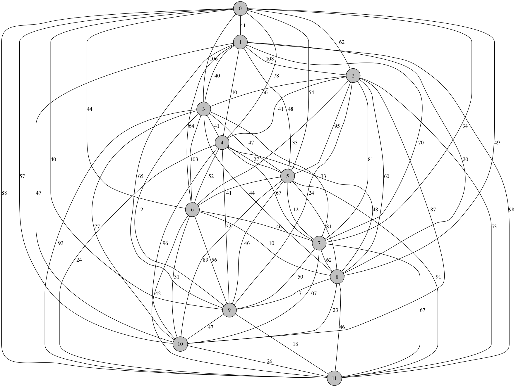
Shortest Route: [0, 7, 5, 4, 1, 8, 6, 10, 11, 9, 3, 2] Distance: 236.0
At 14 nodes, even the efficient algorithm crosses the 1 second threshold.
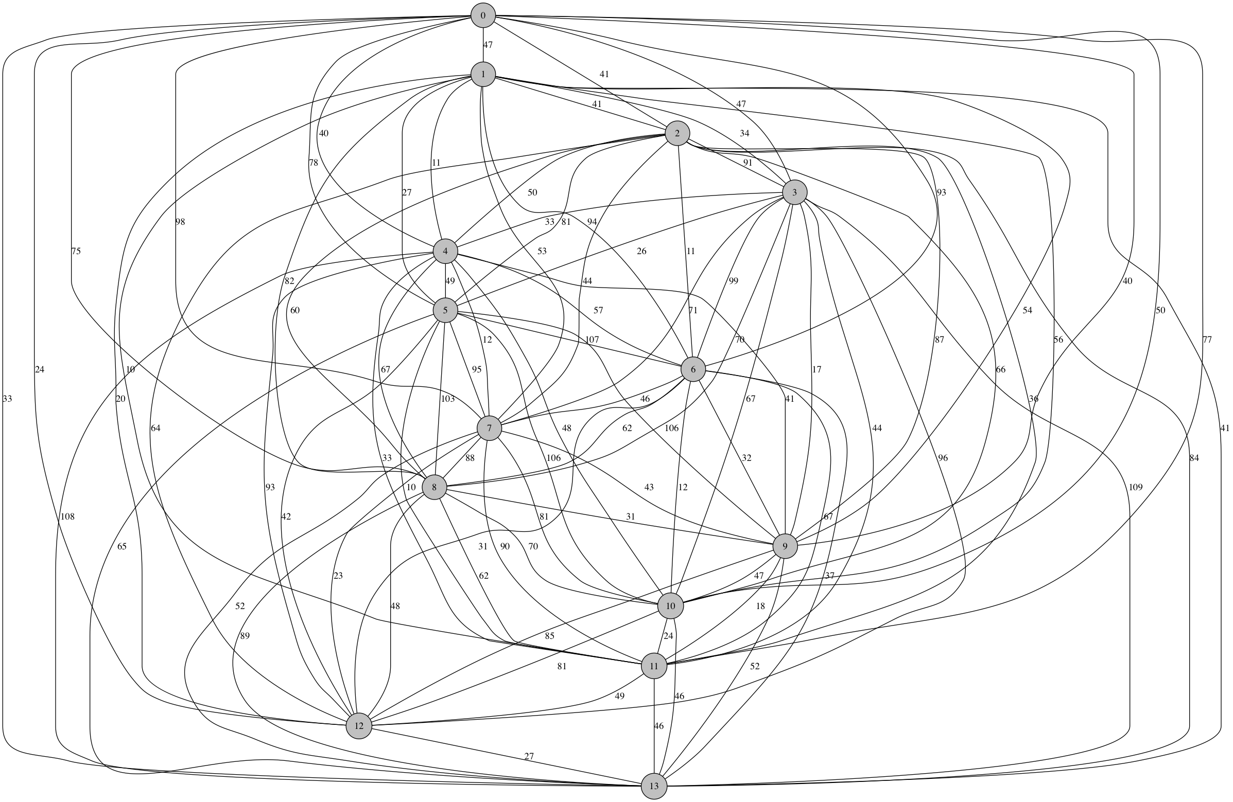
Shortest Route: [0, 2, 6, 10, 13, 12, 7, 4, 1, 11, 5, 3, 9, 8] Distance: 277.0
We tested randomly-generated, fully-connected graphs of up to 18 nodes, and the algorithm was able to compute solutions within a few minutes. Here is an 18-node graph:
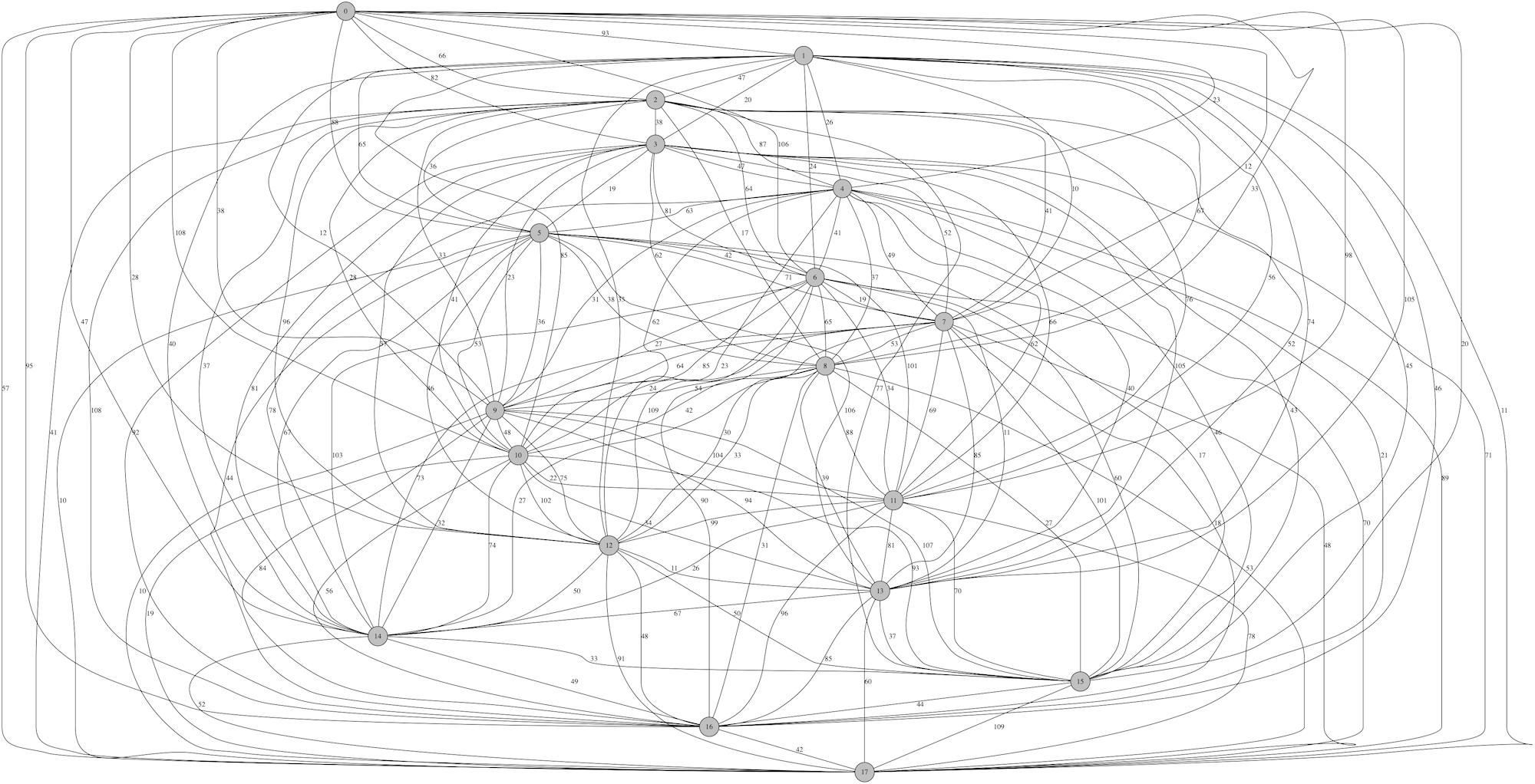
Shortest Route: [0, 3, 10, 6, 12, 5, 11, 2, 14, 8, 13, 4, 7, 1, 9] Distance: 267.0
The Guava TSP Solution
In a prior post we covered the implementation of a solution to the TSP using Guava's Network objects. This implementation utilized a recursive depth-first search algorithm to search for the shortest path among all nodes.
To recap, here was our pseudocode for the TSP solution:
explore(neighbors):

    if(no more unvisited neighbors):
        # This is the base case.
        if total distance is less than current minimum:
            save path and new minimum

    else:
        # This is the recursive case.
        for neighbor in unvisited neighbors:
            visit neighbor
            explore(new_neighbors)
            unvisit neighbor
And here is what the recursive backtracking explore() method looked like
when implemented in Java:
    /** Recursive backtracking method: explore possible solutions starting at this node, having made nchoices */
    public void explore(Node node, int nchoices) {

        if(nchoices == graphSize) {
            //
            // BASE CASE
            //
            if(this.this_distance < this.min_distance || this.min_distance < 0) {
                // Solution base case
                this.min_distance = this.this_distance;
                printSolution();
            }

        } else {
            //
            // RECURSIVE CASE
            //
            Set<Node> neighbors = graph.adjacentNodes(node);
            for(Node neighbor : neighbors) {
                if(neighbor.visited == false) {

                    int distance_btwn = -10000;

                    for( Edge edge : graph.edgesConnecting(node, neighbor) ) {
                        distance_btwn = edge.value;
                    }

                    // Make a choice
                    this.route[nchoices] = neighbor.id;
                    neighbor.visit();
                    this.this_distance += distance_btwn;

                    // Explore the consequences
                    explore(neighbor,nchoices+1);

                    // Unmake the choice
                    this.route[nchoices] = -1;
                    neighbor.unvisit();
                    this.this_distance -= distance_btwn;
                }
                // Move on to the next choice (continue loop)
            }
        } // End base/recursive case
    }
Note: full TSP code available at http://git.charlesreid1.com/charlesreid1/tsp.
Timing the TSP Solution
To time the Guava solution to the TSP, we utilized Java's system time to measure the amount of time it took to compute solutions, excluding the time spent on graph construction.
Here is the code that performs the timing of the call to the explore method:
    public static void main(String[] args) throws IllegalArgumentException {

        ...

        double conn = 1.00;
        TSP t = new TSP(N,conn);

        long start = System.nanoTime();
        t.solve();
        long end = System.nanoTime();
        long duration = end - start;

        System.out.printf("Elapsed time %03f s\n ", (duration/1E9) );
    }
The elapsed time is computed using System.nanoTime().
Writing a script to feed variable size graphs and time the resulting code showed some pretty awful scaling behavior:
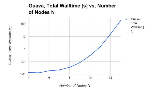
This scaling behavior reveals a bottleneck in the algorithm: the algorithm scales the same way the problem size scales. A more efficient algorithm would be capable of ruling out more of the solution space as the graph size grows, allowing the algorithm to scale better at large problem sizes.
This led to some reconsideration of the algorithm.
Improving the Guava TSP Solution
The original TSP algorithm implemented a subtle flaw - not by implementing a mistake in the calculation, but by ignoring an important piece of information.
The Flaw
As the recursive depth-first search traverses the graph, the algorithm is checking if all nodes have been traversed. When all nodes have been traversed, it then compares the distance of that journey to the current shortest journey. If the new journey is shorter, it is saved as the new shortest journey, otherwise it is ignored and we move on.
What this ignores is the fact that any path, at any point, can be checked to see if it is longer than the current minimum, and if it is, any possibilities that follow from it can be skipped.
For example, consider the TSP on a graph of six cities, A B C D E F.
Suppose that the algorithm is in the midst of the recursive backtracking solution,
and has a current minimum distance and minimum path of the route A-B-E-D-C-F, which is 24 miles.
Now suppose that the algorithm is searching for solutions that begin with the choice A-E-C,
and the distance A-E-C is 28 miles.
The naive algorithm ignores this information, and continues choosing from among the 3 remaining cities, computing the total length for \(3! = 6\) additional routes, and finding that all six of them do not work.
The smart algorithm checks each time it chooses a new node whether the length of the current route exceeds the current minimum route distance (if one has been found/set). If not, the algorithm keeps going, but if so, it skips choosing neighbors and returns directly to the parent caller.
Fixing the Flaw
Fixing the flaw is surpsingly easy: we just add an if statement.
Illustrating first with the pseudocode:
explore(neighbors):

    if(no more unvisited neighbors):
        # This is the base case.
        if total distance is less than current minimum:
            save path and new minimum

    else:
        # This is the recursive case.
        if current distance is greater than current minimum:
            skip
        else:
            for neighbor in unvisited neighbors:
                visit neighbor
                explore(new_neighbors)
                unvisit neighbor
In our Java implementation, the algorithm simply prints out solutions as it goes,
then returns to the calling function whether a solution was found or not.
Thus, we can "skip" a set of solutions by just returning to the calling function,
using a return statement.
        if(nchoices == graphSize) {
            //
            // BASE CASE
            //
            if(this.this_distance < this.min_distance || this.min_distance < 0) {
                // Solution base case:
                this.min_distance = this.this_distance;
                printSolution();
            }

        } else {
            //
            // RECURSIVE CASE
            //

            /*
             * The following lines result in a huge computational cost savings.
            */
            if(this.min_distance>0 && this.this_distance>this.min_distance) {
                // Just give up already. It's meaningless. There's no point.
                return;
            }

            // Everything else stays exactly the same
            Set<Node> neighbors = graph.adjacentNodes(node);
            for(Node neighbor : neighbors) {
                if(neighbor.visited == false) {

                    int distance_btwn = -10000;

                    for( Edge edge : graph.edgesConnecting(node, neighbor) ) {
                        distance_btwn = edge.value;
                    }

                    // Make a choice
                    this.route[nchoices] = neighbor.id;
                    neighbor.visit();
                    this.this_distance += distance_btwn;

                    // Explore the consequences
                    explore(neighbor,nchoices+1);

                    // Unmake the choice
                    this.route[nchoices] = -1;
                    neighbor.unvisit();
                    this.this_distance -= distance_btwn;
                }
                // Move on to the next choice (continue loop)
            }
        } // End base/recursive case
    }
The Pessimist Algorithm
This algorithm is dubbed The Pessimist Algorithm. Let's see how it works. Here is that new if statement:
if(this.min_distance>0 && this.this_distance>this.min_distance) {
    // Just give up already. It's meaningless. There's no point.
    return;
}
This if statement tests two conditions - first, we check if a first minimum distance has actually been found, and second, we check if the distance of the current path is greater than the minimum distance. If it is, we give up continuing our search down this path, and just return back to the calling function.
This introduces a small computational cost -
we now have an if statement to check every time the explore() method is called -
but it results in such significant cost savings that it does not matter.
Timing Results
Shown below is a graph of the walltime for various problem sizes, showing both the original algorithm and the pessimist algorithm and their scaling behavior.
The pessimist algorithm led to a drastic improvement in scale-up - the results are striking.
And here are the results in a table form:
-----------------------------------------------------------------------------------------
| Number of Nodes N | Initial Algorithm Walltime [s] | Pessimist Algorithm Walltime [s] |
|-------------------|--------------------------------|----------------------------------|
| 4                 | 0.005                          | 0.006                            |
| 5                 | 0.006                          | 0.006                            |
| 6                 | 0.009                          | 0.008                            |
| 7                 | 0.017                          | 0.011                            |
| 8                 | 0.029                          | 0.020                            |
| 9                 | 0.083                          | 0.023                            |
| 10                | 0.305                          | 0.053                            |
| 11                | 1.443                          | 0.118                            |
| 12                | 15.808                         | 0.149                            |
| 13                | 180.078                        | 0.524                            |
| 14                |                                | 1.276                            |
| 15                |                                | 3.905                            |
| 16                |                                | 216.827                          |
| 17                |                                | 106.992                          |
| 18                |                                | 337.930                          |
-----------------------------------------------------------------------------------------
For a problem with 13 nodes, the initial algorithm took 3 minutes; the pessimist algorithm didn't even break the one second mark!
Future Work
Now that we've got the algorithm running faster and more efficiently, we can tackle larger problems and explore the impact of problem topology on solutions, and we can rest assured we have an efficient algorithm that can scale to larger and more interesting problems.
There are further improvements we could make to the algorithm to improve it, though. By examining the solutions that are found, we can see that the solutions usually, but not always, connects from each neighbor to its next-closest neighbor. If, when iterating over neighbors, we start by searching the nearest neighbors first, we can potentially get to the minimum solution faster, which would allow us to more quickly rule out larger portions of the solution space that are infeasible.
This would induce an additional overhead cost of sorting, since the Guava library returns the edges that connect to a node as an unordered Set. These edges would have to be added to a container and sorted to implement the nearest-neighbor search.
However, we saw with the pessimist solution that a small increase in complexity can rule out large enough portions of the solution space to make it worthwhile, so it may be that the cost of sorting each edge pays off in the computational savings that result.