- Before We Begin: The Code
- Timing Scripts
- Before You Time: Developing Your Algorithm
- Beginning Your Timing Journey
- Statistical Timing, a.k.a., If You Give A Mouse A Cookie
- Hierarchical Timing Strategy
- Single Problem/Program/Binary
- Multiple Problem/Program/Binary
- Statistical Averaging
- Results
- Summary
Before We Begin: The Code
Note that all of the code discussed/shown in this post is available from the
traveling salesperson problem repository on git.charlesreid1.com.
The guava/ directory contains the guava solution to the traveling salesperson problem,
along with the timing scripts discussed below, and several example output files.
Introduction
Timing a piece of code can be tricky.
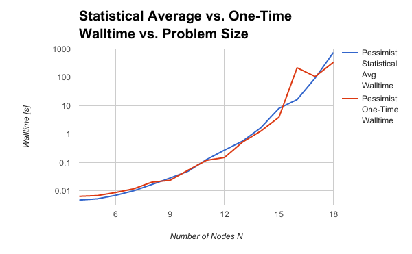
Choosing a random problem of a given size can be problematic, if you happen to randomly chose a particularly easy or difficult case. This can lead to an inaccurate picture of scale-up behavior. Timing results should be statistically averaged - the figure below shows scale-up behavior for the traveling salesperson problem when solving a single random problem, versus a hundred random problems.
This post will cover some conceptual and code tools for measuring the timing and performance of code.
Timing Scripts
Timing a piece of code is a task that sounds simple, on its face. However, the task of profiling code quickly balloons from a single timing of a single bit of code to running hundreds of cases, juggling output from each run, and stitching together script upon script. Soon you find yourself swimming in a pool of output files, looking for your scripts...
In this post we'll cover a workflow for timing a piece of Java code that will help give you a method for thinking about timing. This also balances the need for practicality (i.e., just get it done in as simple a manner as possible) with good design (i.e., flexible inputs and the use of scripts).
Before You Time: Developing Your Algorithm
As you develop your algorithm, you may have variable values hard-coded and random number generators seeding from the same value each time. The intention, as you are developing, is to work out the bugs without the additional difficulty of solving a different problem each time you run the program.
Beginning Your Timing Journey
Once you've implemented your algorithm and verified that it works, the timing portion begins. You can time the code using mechanisms built into the language, which is the most accurate way of timing code. This is called instrumenting your code. To begin with, you might try timing a single problem size, but this information is hard to interpret without more data, so you start to time the code on problems of other sizes.
Here there be dragons.
Statistical Timing, a.k.a., If You Give A Mouse A Cookie
See If You Give A Mouse A Cookie.
Once you time the code solving a single problem, you will want to time the code solving multiple problems.
Once you time the code solving multiple problems, you will want to time the code solving each problem multiple times to get an accurate statistical picture of the solution time on a variety of problems.
Once you get statistics about multiple problem times, you will want to gather statics about variations in problem types and algorithm variations.
It simply does not end. A strategy for managing this deluge of new timing needs prevents spaghetti code.
Hierarchical Timing Strategy
The strategy here is to design code and scripts that are hierarchical. The levels of the hierarchy consist of the different scopes involved in timing: * Single problem/program/binary * Multiple problem/program/binary * Statistical averages using case matrix * Design of Computer Experiments: Testing Variations * Strong and weak scaling (if we decide to continue with parallelization of algorithm)
At each stage, we utilize scripts to bundle the task into a single command or script.
Single Problem/Program/Binary: Makefile
At the scale of solving a single problem, we need a tool that will compile and run Java code - even if it only happens once. Makefiles are an excellent tool for stringing together commands with flags (in the case of the traveling salesperson problem, we need to link to the Guava Jars when we compile and run).
By defining some variables at the top of the Makefile, and a few rules, we have a functional and easy way to build code with scalable complexity:
# Set path to guava
HOME=/Users/charles
GUAVA=$(HOME)/codes/guava/jars/guava-21.0.jar

# Set compile target
BIN=TSP
TARGET=$(BIN).java

# Set java class path
# Hard to believe this actually works, but ok:
CP=-cp '.:$(GUAVA)'


build:
    javac $(CP) $(TARGET)

run:
    # If no size, use default
    java $(CP) $(BIN)

time:
    # Java times itself, we just have to pass it the size
    java $(CP) $(BIN) $(SIZE)

clean:
    rm -rf *.class
Link to code on git.charlesreid1.com
This enables us to run
$ make build
/Users/charles/codes/guava/jars/guava-21.0.jar
and have a new version of the code compile. We can also run a problem with a default size of 5 nodes with a simple make run command:
$ make run
java -cp '.:/Users/charles/codes/guava/jars/guava-21.0.jar' TSP
------------------- TSP Version 2: The Pessimistic Algorithm ----------------------
!!!!!YAY!!!!!!  NEW SOLUTION    Route: [0, 2, 3, 4, 1]  Distance: 258
!!!!!YAY!!!!!!  NEW SOLUTION    Route: [0, 2, 3, 1, 4]  Distance: 257
!!!!!YAY!!!!!!  NEW SOLUTION    Route: [0, 2, 4, 1, 3]  Distance: 189
Found solution...?
Elapsed time 0.005529 s
and have the compiled code run. We can also feed arguments to make commands, and have them passed to the command that is executed:
$ make time SIZE=10
# Java times itself, we just have to pass it the size
java -cp '.:/Users/charles/codes/guava/jars/guava-21.0.jar' TSP 10
------------------- TSP Version 2: The Pessimistic Algorithm ----------------------
!!!!!YAY!!!!!!  NEW SOLUTION    Route: [0, 6, 5, 3, 9, 7, 2, 8, 1, 4]   Distance: 446
!!!!!YAY!!!!!!  NEW SOLUTION    Route: [0, 6, 5, 3, 9, 7, 2, 8, 4, 1]   Distance: 395
!!!!!YAY!!!!!!  NEW SOLUTION    Route: [0, 6, 5, 3, 9, 7, 4, 1, 8, 2]   Distance: 382
!!!!!YAY!!!!!!  NEW SOLUTION    Route: [0, 6, 5, 3, 9, 1, 4, 7, 2, 8]   Distance: 365
!!!!!YAY!!!!!!  NEW SOLUTION    Route: [0, 6, 5, 3, 9, 1, 4, 7, 8, 2]   Distance: 326
!!!!!YAY!!!!!!  NEW SOLUTION    Route: [0, 6, 5, 3, 2, 8, 7, 4, 1, 9]   Distance: 303
!!!!!YAY!!!!!!  NEW SOLUTION    Route: [0, 6, 5, 3, 2, 8, 4, 7, 9, 1]   Distance: 298
!!!!!YAY!!!!!!  NEW SOLUTION    Route: [0, 6, 5, 4, 7, 3, 2, 8, 9, 1]   Distance: 286
!!!!!YAY!!!!!!  NEW SOLUTION    Route: [0, 6, 5, 8, 2, 3, 7, 4, 1, 9]   Distance: 283
!!!!!YAY!!!!!!  NEW SOLUTION    Route: [0, 9, 1, 4, 7, 3, 6, 5, 8, 2]   Distance: 275
!!!!!YAY!!!!!!  NEW SOLUTION    Route: [0, 3, 2, 8, 5, 6, 4, 7, 9, 1]   Distance: 274
!!!!!YAY!!!!!!  NEW SOLUTION    Route: [0, 2, 8, 7, 4, 1, 9, 5, 6, 3]   Distance: 262
!!!!!YAY!!!!!!  NEW SOLUTION    Route: [0, 2, 8, 4, 7, 3, 6, 5, 9, 1]   Distance: 256
Found solution...?
Elapsed time 0.050795 s
For running single cases and gathering small amounts of (initial) timing data, Makefiles greatly simplify the workflow.
Multiple Program/Problem/Binary: Bash
Bash is a faithful scripting language that makes it easy to do simple mechanical tasks like run commands in for loops, necessary for the next level of complexity in our timing hierarchy.
While the task at hand is simple enough, and we could easily use Makefiles, we'll use a separate Bash script for separate functionality and keep things from getting overly complicated in the Makefile.
The essence of the timing script is combining the make time command,
which takes a size parameter, with bash for loops.
Here is a stripped down version of the timing script:
make build

for N in 4 5 6 7 8
do
    make time SIZE=${N}
done
That's it... The rest is just printing!
The make time command passes the size argument on the command line.
The Java Traveling Salesperson Problem code checks if there is an input argument on the command line,
and if there is it uses that as the problem size.
Here's a more embellished script:
export RIGHTNOW="`date +"%Y%m%d_%H%M%S"`"
export OUT="timeout_tsp_java_${RIGHTNOW}.out"
touch ${OUT}
cat /dev/null > ${OUT}

# Compile
make build

for N in {4..8..1}
do
    echo "**************************************" >> ${OUT}
    echo "Running TSP with $N nodes with Java..." >> ${OUT}

    make time SIZE=${N} >> ${OUT} 2>&1

    make dot
    mv graphviz.png graphviz_tsp_${N}.png

    echo "Done." >> ${OUT}

    echo "" >> ${OUT}

done

echo ""
echo ${OUTFILE}
echo ""
Link to code on git.charlesreid1.com
This creates a time-and-date-stamped output file in which all of the output of this script goes - and which can be parsed for plotting the results of timing studies.
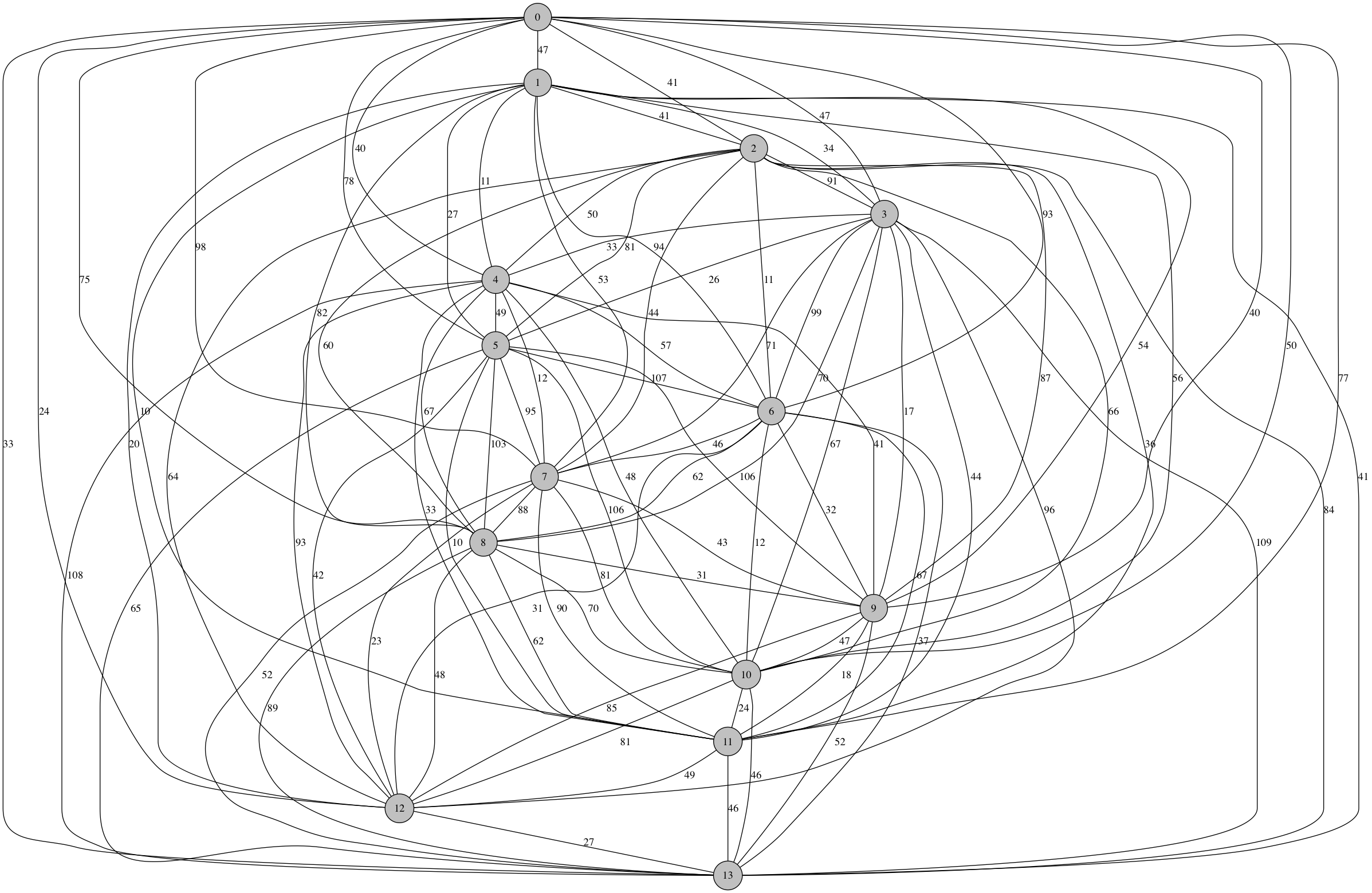
Before it times the solution to the TSP, it dumps out a graphviz dot file containing a schematic of the graph that can be diagrammed:
**************************************
Running TSP with 4 nodes with Java...
Found solution.
Elapsed time 0.004679 s
 Done.

**************************************
Running TSP with 5 nodes with Java...
Found solution.
Elapsed time 0.004543 s
 Done.

**************************************
Running TSP with 6 nodes with Java...
Found solution.
Elapsed time 0.006911 s
 Done.

**************************************
Running TSP with 7 nodes with Java...
Found solution.
Elapsed time 0.008286 s
 Done.

**************************************
Running TSP with 8 nodes with Java...
Found solution.
Elapsed time 0.014499 s
 Done.
In this way we can run a quick test matrix of different problem sizes, and see how the code scales.
Statistical Averaging
Of course, any good computational physicist will tell you that scaling behavior extrapolated from running a single case of a single problem size is folly - your random choice of graph could have been an unusually easy or difficult graph, throwing off the results of the timing.
A proper scaling study really needs to take into account the statistical trends in solution time on a random assortment of problems, so we need a way of scripting solutions to dozens or hundreds of random problems and computing statistically representative measures of code performance.
Our code implements a function to generate random graphs, but for testing and debugging purposes the random number generator was seeded with the same value each time. By making the random number generators truly random, each problem we solve will be a different random graph with the specified number ofn odes.
We can accomplish all of this using bash again: within the for loop over different problem sizes, we will add a for loop for repetitions. Here is the basic framework:
make build

for N in {4..10..1}
do
    for repetition in {0..100..1}
    do
        make time SIZE=${N}
    done
done
And the embellished version that prints the resulting timing information to a file:
# Compile
make build

export RIGHTNOW="`date +"%Y%m%d_%H%M%S"`"

for N in {4..10..1}
do

    export OUT="avgtimeout_tsp_${RIGHTNOW}_${N}.out"
    touch ${OUT}

    echo "**************************************" >> ${OUT}
    echo "Running TSP with $N nodes with Java..." >> ${OUT}

    for repetition in {0..100..1}
    do
        make time SIZE=${N} >> ${OUT} 2>&1
    done
    echo "Done." >> ${OUT}
    echo "" >> ${OUT}

done

echo ""
echo ${OUTFILE}
echo ""
Link to code on git.charlesreid1.com
This results in a file with a large amount of information, but it can be trimmed down to the quantities of interest using a little command line fu. Here are filtered results from an 11-node traveling salesperson problem run approximately 102 times:
$ cat avgtimeout_tsp_20170330_235134_11.out | grep Elapsed | wc -l
     102

$ cat avgtimeout_tsp_20170330_235134_11.out | grep Elapsed
Elapsed time 0.082839 s
Elapsed time 0.130378 s
Elapsed time 0.173737 s
Elapsed time 0.100067 s
Elapsed time 0.166046 s

<clipped>

Elapsed time 0.147801 s
Elapsed time 0.285777 s
Elapsed time 0.078655 s
Elapsed time 0.081246 s
Elapsed time 0.174288 s
Now we have a Makefile that allows us to build and run with a single command, and a bash script that loops over each problem size and runs a set of computations for each problem size. But how to compute an average?
We have an assortment of choices - Python being the most obvious - but in the spirit of
old-school Unix tools like make, cat, grep, and wc, let's use awk to compute the average
walltime for each case size.
Awk to Compute Average Walltime
Given the following output of elapsed walltime for different problem sizes,
$ cat avgtimeout_tsp_20170330_235134_11.out | grep Elapsed
Elapsed time 0.082839 s
Elapsed time 0.130378 s
Elapsed time 0.173737 s
Elapsed time 0.100067 s
Elapsed time 0.166046 s

<clipped>

Elapsed time 0.147801 s
Elapsed time 0.285777 s
Elapsed time 0.078655 s
Elapsed time 0.081246 s
Elapsed time 0.174288 s
we want to extract two things: the first is the problem size (contained in the filename), and the second is the column of numbers.
We can extract the problem size from the filename using sed,
by searching for the pattern _8.out or _10.out.
Here is a Bash one-liner that does this for a variable $f
containing the filename:
N=$(echo $f | sed 's/^.*_\([0-9]\{1,\}\).out/\1/')
The next thing we wnat to do is extract the column of timing data.
This is a good task for the cut utility. We can pass it two flags,
-d to tell it what to use as a field delimiter, and -f to tell it which field
(column) to return. To extract the third column,
cat $f | grep "Elapsed" | cut -d" " -f3
This command results in a series of floating point numbers. If we can pipe it to a program
that can do simple math, like awk, we can compute an average (which is pretty simple math).
Since awk is a text-proecssing program that happens to be able to interpret numbers as numbers,
we have to think like a text processing program. To compute an average, we accumulate the sum
of each line in the file, using an accumulator variable. When we have gone through each line in the file,
we divide this cumulative sum by the number of lines in the file.
cat $f | grep "Elapsed" | cut -d" " -f3 | awk '{a+=$1} END{print a/NR}'
This one-liner uses two important concepts in awk, the first is the bracketed blocks {}
some denoted with BEGIN and END, and the second is the set of built-in variables available in awk.
By surrounding statements by brackets, we denote a block of statements to be run together as the main body of the program.
If the bracket is prefixed by BEFORE, this block of statements is run once at the beginning of the program.
If the bracket is prefixed by END, this block of statements is run once at the end of the program.
To compute an average, the main body of the program is to accumulate a cumulative sum variable.
The END block, run once at the end, is to divide this cumulative sum by the total number of lines.
Finally, these values can be assigned to Bash variables using $(cmd) syntax:
    export N=$(echo $f | sed 's/^.*_\([0-9]\{1,\}\).out/\1/')
    export AVG=$(cat $f | grep "Elapsed" | cut -d" " -f3 | awk '{a+=$1} END{print a/NR}')
    echo "Average time : ${N}-node TSP problem : ${AVG} s"
Here is the final script, which loops over all of the output files generated by the statistical average timing script, which runs 10-100 cases per problem size:
#!/bin/sh

for f in `/bin/ls -1 avgtimeout_tsp*`
do
    touch tmpfile
    cat /dev/null > tmpfile

    export N=$(echo $f | sed 's/^.*_\([0-9]\{1,\}\).out/\1/')
    export AVG=$(cat $f | grep "Elapsed" | cut -d" " -f3 | awk '{a+=$1} END{print a/NR}')
    echo "Average time : ${N}-node TSP problem : ${AVG} s"

    rm tmpfile
done
Link to code on git.charlesreid1.com
Example output:
$ ./avg_calcs.sh  | sort
Average time : 10-node TSP problem : 0.0492826 s
Average time : 11-node TSP problem : 0.125827 s
Average time : 12-node TSP problem : 0.272998 s
Average time : 13-node TSP problem : 0.56743 s
Average time : 14-node TSP problem : 1.24297 s
Average time : 14-node TSP problem : 1.66563 s
Average time : 15-node TSP problem : 8.08373 s
Average time : 16-node TSP problem : 16.4353 s
Average time : 17-node TSP problem : 94.7363 s
Average time : 18-node TSP problem : 749.798 s
Average time : 4-node TSP problem : 0.00473154 s
Average time : 4-node TSP problem : 0.00475648 s
Average time : 5-node TSP problem : 0.005247 s
Average time : 5-node TSP problem : 0.005765 s
Average time : 6-node TSP problem : 0.00694926 s
Average time : 7-node TSP problem : 0.0100795 s
Average time : 8-node TSP problem : 0.0167346 s
Average time : 9-node TSP problem : 0.028239 s
Inspecting the output from particular solutions of particular random graphs shows a wide variation in the number of shortest paths found. For example, for random graphs consisting of 11 nodes, here are some sample solutions. Note the difference in solution times:
------------------- TSP Version 2: The Pessimistic Algorithm ----------------------
NEW SOLUTION    Route: [0, 9, 2, 1, 8, 4, 5, 7, 6, 10, 3]   Distance: 597
NEW SOLUTION    Route: [0, 9, 2, 1, 8, 4, 5, 7, 6, 3, 10]   Distance: 582
NEW SOLUTION    Route: [0, 9, 2, 1, 8, 4, 5, 7, 10, 3, 6]   Distance: 560
NEW SOLUTION    Route: [0, 9, 2, 1, 8, 4, 5, 7, 3, 6, 10]   Distance: 553
NEW SOLUTION    Route: [0, 9, 2, 1, 8, 4, 5, 10, 3, 7, 6]   Distance: 540
NEW SOLUTION    Route: [0, 9, 2, 1, 8, 4, 5, 10, 7, 6, 3]   Distance: 532
NEW SOLUTION    Route: [0, 9, 2, 1, 8, 4, 5, 10, 7, 3, 6]   Distance: 503
NEW SOLUTION    Route: [0, 9, 2, 1, 8, 4, 5, 6, 3, 7, 10]   Distance: 498
NEW SOLUTION    Route: [0, 9, 2, 1, 8, 4, 10, 3, 7, 5, 6]   Distance: 450
NEW SOLUTION    Route: [0, 9, 2, 1, 8, 4, 10, 5, 7, 3, 6]   Distance: 440
NEW SOLUTION    Route: [0, 9, 2, 1, 8, 4, 10, 5, 6, 7, 3]   Distance: 422
NEW SOLUTION    Route: [0, 9, 2, 1, 8, 4, 6, 5, 10, 3, 7]   Distance: 421
NEW SOLUTION    Route: [0, 9, 2, 1, 8, 4, 6, 5, 10, 7, 3]   Distance: 380
NEW SOLUTION    Route: [0, 9, 2, 1, 8, 7, 10, 5, 6, 4, 3]   Distance: 364
NEW SOLUTION    Route: [0, 9, 2, 1, 8, 7, 3, 4, 6, 5, 10]   Distance: 357
NEW SOLUTION    Route: [0, 9, 2, 1, 5, 10, 7, 3, 8, 4, 6]   Distance: 352
NEW SOLUTION    Route: [0, 9, 2, 1, 5, 10, 7, 8, 3, 4, 6]   Distance: 336
NEW SOLUTION    Route: [0, 9, 2, 1, 5, 6, 4, 10, 7, 8, 3]   Distance: 330
NEW SOLUTION    Route: [0, 9, 2, 1, 4, 8, 7, 3, 6, 5, 10]   Distance: 326
NEW SOLUTION    Route: [0, 9, 2, 1, 4, 8, 3, 7, 6, 5, 10]   Distance: 320
NEW SOLUTION    Route: [0, 9, 2, 1, 4, 8, 3, 7, 10, 5, 6]   Distance: 298
NEW SOLUTION    Route: [0, 9, 2, 1, 4, 6, 5, 10, 7, 8, 3]   Distance: 261
NEW SOLUTION    Route: [0, 9, 2, 7, 8, 3, 1, 4, 6, 5, 10]   Distance: 250
NEW SOLUTION    Route: [0, 9, 8, 7, 2, 3, 1, 4, 6, 5, 10]   Distance: 245
Found solution.
Elapsed time 0.057047 s

------------------- TSP Version 2: The Pessimistic Algorithm ----------------------
NEW SOLUTION    Route: [0, 8, 1, 6, 4, 9, 10, 5, 2, 7, 3]   Distance: 650
NEW SOLUTION    Route: [0, 8, 1, 6, 4, 9, 10, 5, 2, 3, 7]   Distance: 641
NEW SOLUTION    Route: [0, 8, 1, 6, 4, 9, 10, 5, 7, 2, 3]   Distance: 638
NEW SOLUTION    Route: [0, 8, 1, 6, 4, 9, 10, 5, 7, 3, 2]   Distance: 630
NEW SOLUTION    Route: [0, 8, 1, 6, 4, 9, 10, 7, 5, 2, 3]   Distance: 589
NEW SOLUTION    Route: [0, 8, 1, 6, 4, 9, 10, 2, 3, 7, 5]   Distance: 580
NEW SOLUTION    Route: [0, 8, 1, 6, 4, 9, 10, 2, 5, 7, 3]   Distance: 548
NEW SOLUTION    Route: [0, 8, 1, 6, 4, 9, 2, 5, 7, 3, 10]   Distance: 533
NEW SOLUTION    Route: [0, 8, 1, 6, 4, 9, 7, 5, 2, 3, 10]   Distance: 522
NEW SOLUTION    Route: [0, 8, 1, 6, 4, 9, 7, 5, 2, 10, 3]   Distance: 495
NEW SOLUTION    Route: [0, 8, 1, 6, 7, 9, 4, 5, 2, 10, 3]   Distance: 494
NEW SOLUTION    Route: [0, 8, 1, 6, 7, 5, 4, 9, 2, 10, 3]   Distance: 493
NEW SOLUTION    Route: [0, 8, 1, 6, 3, 10, 2, 5, 7, 9, 4]   Distance: 490
NEW SOLUTION    Route: [0, 8, 1, 6, 3, 10, 2, 5, 7, 4, 9]   Distance: 486
NEW SOLUTION    Route: [0, 8, 1, 6, 9, 4, 7, 5, 2, 10, 3]   Distance: 467
NEW SOLUTION    Route: [0, 8, 1, 10, 2, 5, 7, 4, 9, 6, 3]   Distance: 453
NEW SOLUTION    Route: [0, 8, 1, 2, 5, 7, 4, 9, 6, 3, 10]   Distance: 442
NEW SOLUTION    Route: [0, 8, 1, 2, 5, 7, 4, 9, 6, 10, 3]   Distance: 437
NEW SOLUTION    Route: [0, 8, 1, 5, 7, 4, 9, 2, 10, 6, 3]   Distance: 433
NEW SOLUTION    Route: [0, 8, 10, 2, 1, 5, 4, 9, 7, 6, 3]   Distance: 427
NEW SOLUTION    Route: [0, 8, 10, 2, 1, 5, 7, 4, 9, 6, 3]   Distance: 400
NEW SOLUTION    Route: [0, 8, 2, 1, 5, 7, 4, 9, 6, 10, 3]   Distance: 399
NEW SOLUTION    Route: [0, 3, 7, 4, 9, 6, 10, 2, 1, 5, 8]   Distance: 394
NEW SOLUTION    Route: [0, 3, 7, 4, 9, 6, 10, 2, 8, 5, 1]   Distance: 389
NEW SOLUTION    Route: [0, 3, 6, 9, 4, 7, 5, 8, 1, 2, 10]   Distance: 384
NEW SOLUTION    Route: [0, 3, 6, 9, 4, 7, 5, 8, 10, 2, 1]   Distance: 382
NEW SOLUTION    Route: [0, 3, 6, 9, 4, 7, 5, 1, 2, 8, 10]   Distance: 374
NEW SOLUTION    Route: [0, 9, 4, 5, 1, 2, 8, 10, 3, 6, 7]   Distance: 373
NEW SOLUTION    Route: [0, 9, 4, 7, 3, 6, 10, 8, 5, 1, 2]   Distance: 365
NEW SOLUTION    Route: [0, 9, 4, 7, 3, 6, 10, 2, 1, 5, 8]   Distance: 360
NEW SOLUTION    Route: [0, 9, 4, 7, 3, 6, 10, 2, 8, 5, 1]   Distance: 355
NEW SOLUTION    Route: [0, 9, 4, 7, 5, 8, 1, 2, 10, 6, 3]   Distance: 345
NEW SOLUTION    Route: [0, 9, 4, 7, 5, 1, 2, 8, 10, 6, 3]   Distance: 335
Found solution.
Elapsed time 0.159882 s

------------------- TSP Version 2: The Pessimistic Algorithm ----------------------
NEW SOLUTION    Route: [0, 3, 10, 2, 5, 4, 7, 8, 1, 9, 6]   Distance: 500
NEW SOLUTION    Route: [0, 3, 10, 2, 5, 4, 7, 8, 1, 6, 9]   Distance: 498
NEW SOLUTION    Route: [0, 3, 10, 2, 5, 4, 7, 8, 6, 1, 9]   Distance: 493
NEW SOLUTION    Route: [0, 3, 10, 2, 5, 4, 7, 8, 6, 9, 1]   Distance: 481
NEW SOLUTION    Route: [0, 3, 10, 2, 5, 4, 7, 8, 9, 1, 6]   Distance: 443
NEW SOLUTION    Route: [0, 3, 10, 2, 5, 4, 7, 8, 9, 6, 1]   Distance: 429
NEW SOLUTION    Route: [0, 3, 10, 2, 5, 6, 1, 9, 8, 7, 4]   Distance: 417
NEW SOLUTION    Route: [0, 3, 10, 2, 6, 5, 4, 7, 8, 9, 1]   Distance: 360
NEW SOLUTION    Route: [0, 3, 10, 2, 1, 9, 6, 5, 4, 7, 8]   Distance: 359
NEW SOLUTION    Route: [0, 3, 10, 4, 5, 6, 2, 1, 9, 7, 8]   Distance: 358
NEW SOLUTION    Route: [0, 3, 10, 4, 5, 6, 2, 1, 9, 8, 7]   Distance: 342
NEW SOLUTION    Route: [0, 3, 10, 4, 5, 6, 9, 8, 7, 2, 1]   Distance: 340
NEW SOLUTION    Route: [0, 3, 10, 4, 7, 8, 9, 1, 2, 6, 5]   Distance: 310
NEW SOLUTION    Route: [0, 3, 7, 8, 9, 10, 4, 5, 6, 2, 1]   Distance: 305
NEW SOLUTION    Route: [0, 3, 9, 8, 7, 4, 10, 1, 2, 6, 5]   Distance: 303
NEW SOLUTION    Route: [0, 5, 4, 7, 3, 10, 8, 9, 6, 2, 1]   Distance: 301
NEW SOLUTION    Route: [0, 5, 4, 7, 3, 10, 1, 2, 6, 9, 8]   Distance: 293
NEW SOLUTION    Route: [0, 5, 4, 7, 3, 1, 6, 2, 10, 9, 8]   Distance: 286
NEW SOLUTION    Route: [0, 5, 4, 7, 3, 1, 2, 6, 9, 10, 8]   Distance: 281
NEW SOLUTION    Route: [0, 5, 4, 7, 3, 1, 2, 6, 10, 9, 8]   Distance: 275
NEW SOLUTION    Route: [0, 5, 4, 7, 8, 9, 6, 2, 1, 3, 10]   Distance: 270
NEW SOLUTION    Route: [0, 5, 4, 7, 8, 9, 10, 3, 1, 2, 6]   Distance: 269
NEW SOLUTION    Route: [0, 5, 4, 10, 3, 7, 8, 9, 6, 2, 1]   Distance: 268
NEW SOLUTION    Route: [0, 5, 4, 10, 9, 8, 7, 3, 1, 2, 6]   Distance: 252
NEW SOLUTION    Route: [0, 5, 4, 10, 9, 6, 2, 1, 3, 7, 8]   Distance: 248
NEW SOLUTION    Route: [0, 5, 6, 2, 10, 4, 7, 8, 9, 3, 1]   Distance: 235
NEW SOLUTION    Route: [0, 5, 6, 2, 1, 3, 10, 4, 7, 8, 9]   Distance: 231
NEW SOLUTION    Route: [0, 5, 6, 2, 1, 3, 7, 4, 10, 9, 8]   Distance: 212
NEW SOLUTION    Route: [0, 5, 6, 2, 1, 3, 9, 10, 4, 7, 8]   Distance: 207
Found solution.
Elapsed time 0.175282 s

------------------- TSP Version 2: The Pessimistic Algorithm ----------------------
NEW SOLUTION    Route: [0, 6, 7, 2, 5, 10, 4, 9, 3, 8, 1]   Distance: 515
NEW SOLUTION    Route: [0, 6, 7, 2, 5, 10, 4, 9, 3, 1, 8]   Distance: 495
NEW SOLUTION    Route: [0, 6, 7, 2, 5, 10, 4, 9, 8, 1, 3]   Distance: 423
NEW SOLUTION    Route: [0, 6, 7, 2, 5, 10, 4, 8, 9, 1, 3]   Distance: 368
NEW SOLUTION    Route: [0, 6, 7, 2, 5, 10, 4, 3, 8, 9, 1]   Distance: 361
NEW SOLUTION    Route: [0, 6, 7, 2, 5, 10, 4, 3, 1, 9, 8]   Distance: 341
NEW SOLUTION    Route: [0, 6, 7, 2, 5, 1, 9, 8, 3, 4, 10]   Distance: 330
NEW SOLUTION    Route: [0, 6, 7, 2, 10, 5, 1, 9, 8, 4, 3]   Distance: 309
NEW SOLUTION    Route: [0, 6, 7, 10, 2, 5, 1, 9, 8, 4, 3]   Distance: 284
NEW SOLUTION    Route: [0, 6, 7, 8, 9, 1, 5, 2, 10, 4, 3]   Distance: 266
NEW SOLUTION    Route: [0, 6, 7, 8, 9, 1, 5, 10, 2, 4, 3]   Distance: 258
NEW SOLUTION    Route: [0, 6, 5, 2, 10, 4, 3, 1, 9, 8, 7]   Distance: 250
NEW SOLUTION    Route: [0, 6, 5, 2, 10, 7, 8, 9, 1, 3, 4]   Distance: 243
NEW SOLUTION    Route: [0, 6, 5, 2, 4, 3, 1, 9, 8, 7, 10]   Distance: 225
NEW SOLUTION    Route: [0, 6, 5, 1, 9, 8, 7, 10, 2, 4, 3]   Distance: 197
Found solution.
Elapsed time 0.051783 s

------------------- TSP Version 2: The Pessimistic Algorithm ----------------------
NEW SOLUTION    Route: [0, 8, 9, 6, 1, 7, 3, 4, 5, 2, 10]   Distance: 607
NEW SOLUTION    Route: [0, 8, 9, 6, 1, 7, 3, 4, 2, 5, 10]   Distance: 573
NEW SOLUTION    Route: [0, 8, 9, 6, 1, 7, 3, 4, 10, 5, 2]   Distance: 562
NEW SOLUTION    Route: [0, 8, 9, 6, 1, 7, 3, 5, 2, 4, 10]   Distance: 513
NEW SOLUTION    Route: [0, 8, 9, 6, 1, 3, 5, 2, 7, 4, 10]   Distance: 496
NEW SOLUTION    Route: [0, 8, 9, 6, 7, 3, 1, 5, 2, 4, 10]   Distance: 493
NEW SOLUTION    Route: [0, 8, 9, 6, 7, 3, 1, 10, 4, 2, 5]   Distance: 489
NEW SOLUTION    Route: [0, 8, 9, 6, 7, 2, 4, 10, 1, 3, 5]   Distance: 487
NEW SOLUTION    Route: [0, 8, 9, 6, 7, 2, 5, 3, 1, 10, 4]   Distance: 480
NEW SOLUTION    Route: [0, 8, 9, 6, 4, 3, 5, 2, 7, 1, 10]   Distance: 454
NEW SOLUTION    Route: [0, 8, 9, 6, 4, 5, 2, 7, 3, 1, 10]   Distance: 453
NEW SOLUTION    Route: [0, 8, 9, 6, 4, 10, 5, 2, 7, 3, 1]   Distance: 452
NEW SOLUTION    Route: [0, 8, 9, 6, 4, 10, 1, 7, 3, 5, 2]   Distance: 443
NEW SOLUTION    Route: [0, 8, 9, 6, 4, 10, 1, 3, 5, 2, 7]   Distance: 411
NEW SOLUTION    Route: [0, 8, 9, 10, 4, 6, 1, 3, 5, 2, 7]   Distance: 407
NEW SOLUTION    Route: [0, 8, 9, 10, 4, 6, 7, 2, 5, 3, 1]   Distance: 402
NEW SOLUTION    Route: [0, 8, 9, 10, 4, 6, 5, 2, 7, 3, 1]   Distance: 390
NEW SOLUTION    Route: [0, 8, 9, 10, 4, 6, 2, 7, 3, 1, 5]   Distance: 388
NEW SOLUTION    Route: [0, 8, 9, 10, 4, 6, 2, 7, 1, 3, 5]   Distance: 387
NEW SOLUTION    Route: [0, 8, 9, 10, 4, 6, 2, 5, 3, 1, 7]   Distance: 384
NEW SOLUTION    Route: [0, 8, 9, 10, 1, 3, 5, 2, 7, 4, 6]   Distance: 376
NEW SOLUTION    Route: [0, 8, 9, 10, 6, 4, 3, 1, 7, 2, 5]   Distance: 371
NEW SOLUTION    Route: [0, 8, 9, 10, 6, 4, 3, 1, 5, 2, 7]   Distance: 367
NEW SOLUTION    Route: [0, 8, 9, 10, 6, 4, 2, 5, 3, 1, 7]   Distance: 366
NEW SOLUTION    Route: [0, 8, 9, 10, 6, 4, 7, 2, 5, 3, 1]   Distance: 365
NEW SOLUTION    Route: [0, 8, 9, 5, 3, 1, 10, 6, 4, 2, 7]   Distance: 358
NEW SOLUTION    Route: [0, 8, 9, 5, 2, 7, 3, 1, 10, 4, 6]   Distance: 352
NEW SOLUTION    Route: [0, 8, 2, 4, 6, 10, 9, 5, 3, 7, 1]   Distance: 344
NEW SOLUTION    Route: [0, 8, 2, 4, 6, 10, 9, 5, 3, 1, 7]   Distance: 328
NEW SOLUTION    Route: [0, 8, 2, 7, 3, 1, 5, 9, 10, 4, 6]   Distance: 321
NEW SOLUTION    Route: [0, 8, 2, 7, 1, 3, 5, 9, 10, 4, 6]   Distance: 320
NEW SOLUTION    Route: [0, 8, 5, 3, 1, 9, 10, 6, 4, 2, 7]   Distance: 319
NEW SOLUTION    Route: [0, 8, 5, 9, 10, 6, 4, 2, 7, 3, 1]   Distance: 314
NEW SOLUTION    Route: [0, 8, 5, 2, 7, 3, 1, 9, 10, 4, 6]   Distance: 313
NEW SOLUTION    Route: [0, 8, 4, 3, 5, 2, 7, 1, 9, 10, 6]   Distance: 299
NEW SOLUTION    Route: [0, 8, 4, 3, 7, 2, 5, 9, 1, 10, 6]   Distance: 293
NEW SOLUTION    Route: [0, 8, 4, 3, 1, 7, 2, 5, 9, 10, 6]   Distance: 278
NEW SOLUTION    Route: [0, 8, 4, 2, 7, 3, 1, 5, 9, 10, 6]   Distance: 277
NEW SOLUTION    Route: [0, 8, 4, 2, 7, 1, 3, 5, 9, 10, 6]   Distance: 276
NEW SOLUTION    Route: [0, 8, 4, 6, 10, 9, 5, 3, 1, 7, 2]   Distance: 263
NEW SOLUTION    Route: [0, 8, 4, 6, 10, 9, 5, 3, 1, 2, 7]   Distance: 262
NEW SOLUTION    Route: [0, 8, 4, 6, 10, 9, 5, 2, 7, 3, 1]   Distance: 249
NEW SOLUTION    Route: [0, 3, 5, 9, 10, 6, 4, 8, 1, 7, 2]   Distance: 245
NEW SOLUTION    Route: [0, 3, 5, 9, 10, 6, 4, 8, 1, 2, 7]   Distance: 244
NEW SOLUTION    Route: [0, 3, 7, 2, 5, 9, 10, 1, 8, 4, 6]   Distance: 242
NEW SOLUTION    Route: [0, 3, 7, 2, 5, 9, 10, 6, 4, 8, 1]   Distance: 231
NEW SOLUTION    Route: [0, 3, 1, 8, 4, 6, 10, 9, 5, 2, 7]   Distance: 215
Found solution.
Elapsed time 0.087109 s
Results
The figure below shows the results of the timing study when using the average of 100 different random problems, compared to the timing study performed using a single problem size.
The results show dramatically different behavior, highlighting the importance of computing the statistical average of solution walltime for many different problems. This was not an issue that arose in discussing timing or profiling of codes to solve the 8 queens problem, because in that case the problem (and resulting decision tree) were determined by the choice of algorithm.
This information is also important ot keep in mind when comparing the timing performance of two algorithms - using many cases to compare two algorithms is preferrable, since it reduces the likelihood of randomly selecting a problem that highights a weakness of one algorithm or a strength of the other.
Summary
In this post we covered some scripting tools that make timing a lot easier to do, and some ways of thinking about and building up scripts to allow for more complex timing studies without an increase in the associated post-processing work involved.
We showed how to use make and a Makefile to create compact, expressive commands to build and run Java programs.
We showed how to use Bash scripting to implement loops and run a case matrix of problems of various sizes,
measuring timing data for hundreds of problems in total.
All of these scripts made heavy use of Unix command line tools,
demonstrating how to chain commands and functionality together on the command line to accomplish complex tasks.
Finally, we showed how to use the awk programming language to compute the average of a set of numbers,
exploring yet another application of this unusually handy language.