This is Part 1 of a 4-part blog post on the mathematics of the 4x4 Rubik's Cube, its relation to algorithms, and some curious properties of Rubik's Cubes.

You are currently reading Part 1 of this blog post: Part 1: Representations

See Part 2 of this blog post here: Part 2: Permutations

See Part 3 of this blog post here: Part 3: Factoring Permutations

See Part 4 of this blog post here: Part 4: Sequence Order

Table of Contents

• Introduction: Why the Rubik's Cube

  • Why the 4x4 Rubik's Cube

• How the Rubik's Cube Works

  • The Pieces
  • Face Notation
  • Color Notation
  • Move Notation
    • Regular Face Rotations
    • Reverse Face Rotations
    • Double Face Rotations
    • Second Layer Face Rotations

• Computer Representation of a Rubik's Cube

  • Operations and Functionality
  • Face Numbering

• Tuple

  • Tuple Representation Requirements
  • Tuple Representation

• Preview of Part 2

• References

Introduction: Why The Rubik's Cube

In this series of four posts, we'll take a look at the 4x4 Rubik's Cube. The Rubik's Cube is an interesting puzzle that has some profound mathematical connections to group theory and combinatorics.

Group theory is a branch of mathematics that applies to any system that exhibits symmetry; combinatorics is the mathematics of counting things.

The Rubik's Cube gives us the opportunity to apply concepts in group theory and combinatorics to better understand how the cube works, and to learn how to apply these principles to real world systems.

Finally, we will wrap up by discussing some of the algorithms that are required to deal with a Rubik's Cube computationally.

In the next two posts, we'll talk more about the mathematical representation of permutations of the Rubik's Cube, and how to use this representation to understand some of the properties of move sequences when applied to the cube.

Why The 4x4 Rubik's Cube

The 4x4 Rubik's cube, also known as the Rubik's Revenge cube, is larger than the standard 3x3 Rubik's Cube - 96 faces, instead of the ususal 36. The 4x4 cube exhibits some particularly interesting properties as a result of having an even number of squares on each edge.

How the Rubik's Cube Works

Let's start with a discussion of cube mechanics, since this is important to coming up with an accurate mathematical model of the cube.

The Pieces

The 4x4 Rubik's Cube consists of six faces of sixteen squares each, for a total of 96 face squares. These face squares are not completely interchangeable, however - the 4x4 cube is actually composed of three types of pieces, called "cubies".

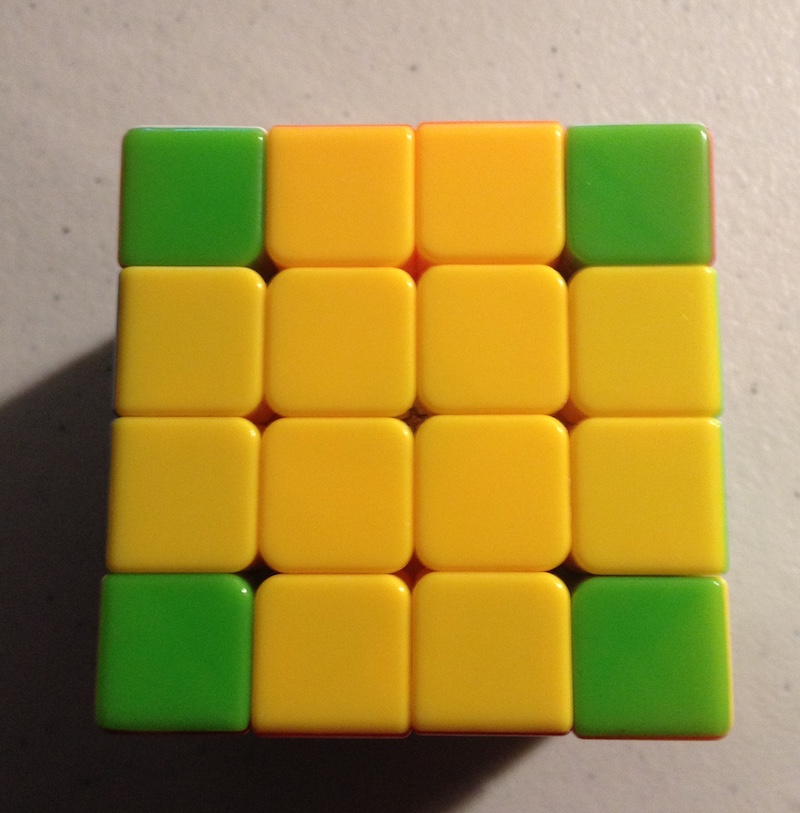
Figure 1: Corner pieces are green.

The first type of piece is a corner piece, which contains 3 faces. Note that it is impossible for the corner pieces to change their chirality (direction of rotation). There are 8 corner pieces, each of which can be oriented in 3 different ways.

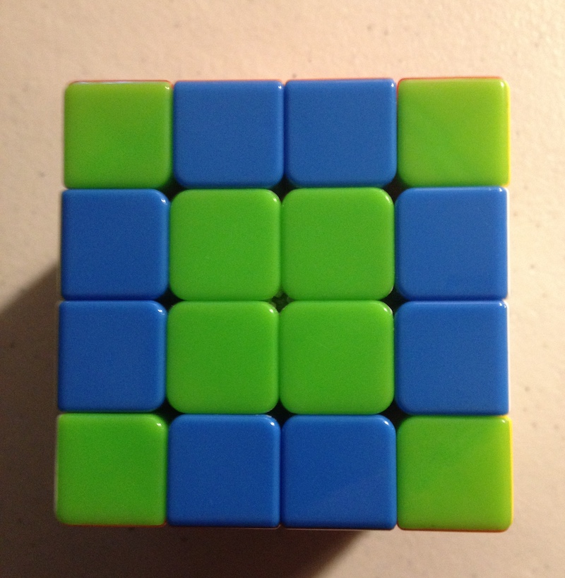
Figure 2: Double edge pieces are blue.

The second type of piece is a double edge (dedge) piece. Each edge is composed of two double edges. There are 24 total double edge pieces, which can be further classified into 12 left-handed and 12 right-handed dedge pieces.

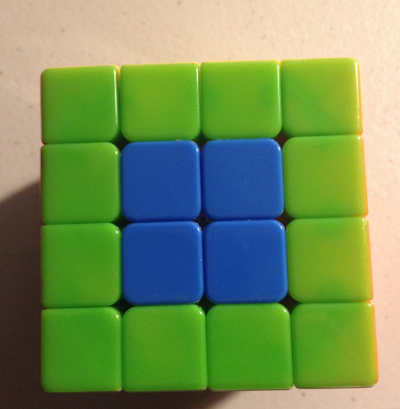
Figure 3: Center pieces are blue.

Lastly, there are 4 center pieces in the center of each face, for a total of 24 center pieces. Note that each of the center pieces of a given color are interchangeable, unlike the double edge pieces or corners.

Face Notation

To refer to particular faces on the cube, we use six letters to indicate different faces:

U - upper face (the top of the cube)

D - downward face (the bottom of the cube0

F - front face (the front of the cube)

B - back face (the back side of the cube)

L - left face of the cube (on the left side when facing the front F face)

R - right face of the cube

This will help refer to how we will rotate the cube.

Color Notation

In the solved state, each cube face has one of six colors. The orientation of these colors relative to one another is always fixed; the red and orange colored faces, for example, are never adjacent. This is due to the nature of the mechanical pieces that compose the Rubik's Cube.

The standard faces for each color on a solved cube are:

• U = White
• D = Yellow
• F = Green
• B = Blue (Back-Blue)
• L = Orange
• R = Red (Red-Right)

Note that on a 3x3 cube, we can always determine the final color a face will have, because the six center pieces on each side of a 3x3 cube always remain fixed.

On a 4x4 cube, however, all four center squares can rotate and move, meaning all 24 center squares are totally interchangeable, and there is no link between the center colors on a 4x4 cube and the final color that will be on that face when the cube is solved.

Move Notation

Using the face notation explained above, we can denote multiple types of moves on the 4x4 Rubik's Cube.

We have 36 total moves that we can make on the 4x4 Rubik's Cube, which can be grouped by the dozen:

L l r R
U u d D
B b f F

L' l' r' R'
U' u' d' D'
B' b' f' F'

2L 2L' 2R 2R'
2U 2U' 2D 2D'
2B 2B' 2F 2F'

Let's go through the details of the notation.

Regular Face Rotations

The regular face turns are denoted with capital letters: L R U D B F refer to a single clockwise rotation of the respective face. Here, "clockwise" means the direction that is clockwise when facing the given face head-on.

Reverse Face Rotations

The ' apostrophe following moves, as in L' R' U' D' B' F', indicates that the move shoud be a counter-clockwise rotation of the given face, instead of clockwise.

Double Face Rotations

Rotations that are indicated using a lowercase letter refer to two-layer rotations: l r u d b f.

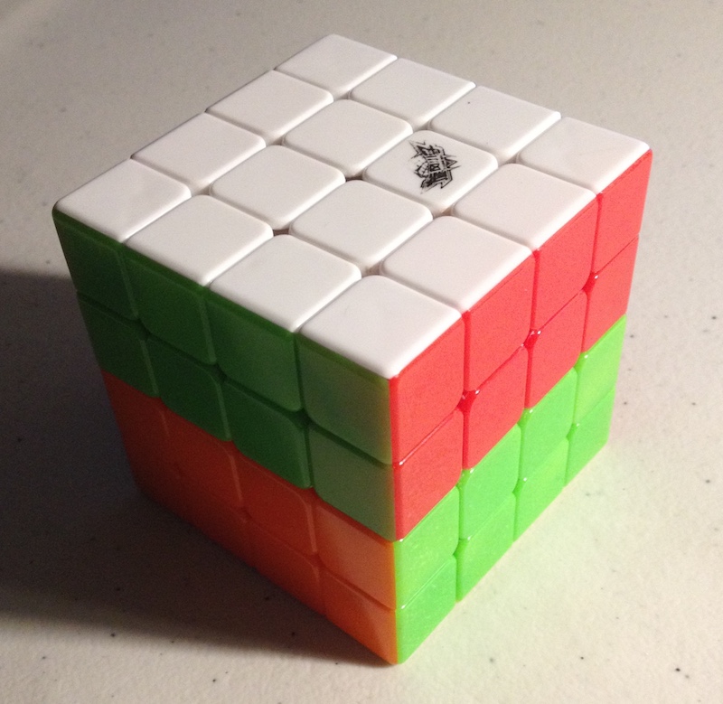
Figure 4: Cube state after move u.

That is, the lowercase u refers to the clockwise rotation of the top two layers of the cube; the lowercase r refers to the clockwise rotation of the rightmost two layers of the cube; and so on.

The apostrophe also serves to indicate a counter-clockwise rotation: 'l r' u' d' b' f' indicate counter clockwise rotations of the two left, two right, two upper, two bottom, two back, and two front layers, respectively.

We have covered the first 24 moves - clockwise and counter-clockwise rotations of single and double layers.

Second Layer Face Rotations

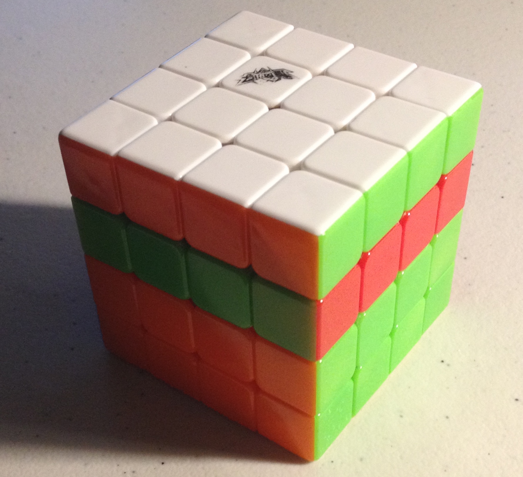
Figure 5: Cube state after move 2U.

The 2 notation indicates a rotation of the second layer only. For example, 2U refers to the clockwise rotation of the second layer from the top. This is equivalent to the move sequence u U'.

Likewise, the apostrophe indicates a counterclockwise rotation.

Computer Representation of a Rubik's Cube

The computer representation we are using is the rubiks-cube-NxNxN-solver library by Github user @dwalton.

We have modified this library to provide additional functionality needed in the project; the fork used in this project is available at git.charlesreid1.com: rubiks-cube-nnn-solver

Using this library, here's how we create a 4x4 Rubik's Revenge cube:

In [1]: from rubikscubennnsolver.RubiksCube444 import RubiksCube444, solved_4x4x4

In [2]: order = 'URFDLB'

In [3]: cube = RubiksCube444(solved_4x4x4, order)

In [4]: cube.print_cube()
         U U U U
         U U U U
         U U U U
         U U U U

L L L L  F F F F  R R R R  B B B B
L L L L  F F F F  R R R R  B B B B
L L L L  F F F F  R R R R  B B B B
L L L L  F F F F  R R R R  B B B B

         D D D D
         D D D D
         D D D D
         D D D D

Operations and Functionality

Some important functionality:

• Obtaining each side
• Applying rotation
• Applying sequence of rotations
• Each side
• Side face numberings, centers, edges

To obtain each side, use the sides attribute:

In [8]: print(cube.sides)
OrderedDict([('U', <rubikscubennnsolver.RubiksSide.Side object at 0x11172d358>), 
             ('L', <rubikscubennnsolver.RubiksSide.Side object at 0x11172d240>), 
             ('F', <rubikscubennnsolver.RubiksSide.Side object at 0x11172d5c0>), 
             ('R', <rubikscubennnsolver.RubiksSide.Side object at 0x11172d5f8>), 
             ('B', <rubikscubennnsolver.RubiksSide.Side object at 0x11172d518>), 
             ('D', <rubikscubennnsolver.RubiksSide.Side object at 0x11172d390>)])

Each Side object has a long list of methods, including methods to obtain the index numbers of corner, edge, or center faces on a particular side.

To apply a rotation of a single face, use the rotate() method and pass the name of the face:

In [10]: cube.rotate("U")

In [11]: cube.print_cube()
         U U U U
         U U U U
         U U U U
         U U U U

F F F F  R R R R  B B B B  L L L L
L L L L  F F F F  R R R R  B B B B
L L L L  F F F F  R R R R  B B B B
L L L L  F F F F  R R R R  B B B B

         D D D D
         D D D D
         D D D D
         D D D D

Unfortunately, the rotate method does not take sequences of moves, but this is easily resolved:

In [12]: cube = RubiksCube444(solved_4x4x4, order)

In [13]: sequence = "U L U' L'"

In [14]: for move in sequence.split():
    ...:     cube.rotate(move)
    ...:

In [15]: cube.print_cube()
         L U U U
         U U U U
         U U U U
         U B B L

D F F F  R L L F  U R R R  B B B B
L L L L  F F F F  R R R R  B B B U
L L L L  F F F F  R R R R  B B B U
L L L L  F F F F  R R R R  B B B U

         D D D D
         D D D D
         D D D D
         B D D D

Face Numbering

Here is the numerical representation of the faces, which we will make extensive use of:

In [6]: cube.print_cube_layout()
             01 02 03 04
             05 06 07 08
             09 10 11 12
             13 14 15 16

17 18 19 20  33 34 35 36  49 50 51 52  65 66 67 68
21 22 23 24  37 38 39 40  53 54 55 56  69 70 71 72
25 26 27 28  41 42 43 44  57 58 59 60  73 74 75 76
29 30 31 32  45 46 47 48  61 62 63 64  77 78 79 80

             81 82 83 84
             85 86 87 88
             89 90 91 92
             93 94 95 96

Tuple Representation

We have a goal of finding a way of representing the state of the 4x4 Rubik's Revenge using a tuple, which is a mathematical object that will enable us to investigate properties of sequences, moves, and rotations.

It is important to note that the mechanics of the cube restrict some of the 96 total faces to only occur in particular configurations. By using a tuple of 96 integers, we are overspecifying the state of the cube, and we would be able to do much better if our goal were a minimal representation of the Rubik's Cube state.

However, our goal is not a minimal representation of the cube, but a unique representation of the cube. As we will see in a later post, the schema we use does not actually matter, so long as we can represent each unique state of the cube using a sequence of integers of arbitrary length.

Tuple Representation Requirements

The 4x4 cube, in the solved state, has a few characteristics that can be used to indicate a particular permutation or configuration:

• Face indciators UDFBLR
• Colors WYGBRO
• Integers 1-96 to number each face

Here is how the faces representation looks:

In [17]: cube.print_cube()
         U U U U
         U U U U
         U U U U
         U U U U

L L L L  F F F F  R R R R  B B B B
L L L L  F F F F  R R R R  B B B B
L L L L  F F F F  R R R R  B B B B
L L L L  F F F F  R R R R  B B B B

         D D D D
         D D D D
         D D D D
         D D D D

The equivalent color representation is:

         W W W W
         W W W W
         W W W W
         W W W W

O O O O  G G G G  R R R R  B B B B
O O O O  G G G G  R R R R  B B B B
O O O O  G G G G  R R R R  B B B B
O O O O  G G G G  R R R R  B B B B

         Y Y Y Y
         Y Y Y Y
         Y Y Y Y
         Y Y Y Y

However, the tuple representation cannot use colors to represent the state of the cube. This is because a tuple representation using "R" to represent each red face would give us no way of distinguishing between the (non-interchangeable) red faces on the cube. For example, if the red-green double edge piece were replaced with a red-blue double edge piece, oriented with the red face at the same location, the n-tuple needs to reflect that this face has a different value than it did the prior move.

For this reason, we must use an integer to index each distinct face:

             01 02 03 04
             05 06 07 08
             09 10 11 12
             13 14 15 16

17 18 19 20  33 34 35 36  49 50 51 52  65 66 67 68
21 22 23 24  37 38 39 40  53 54 55 56  69 70 71 72
25 26 27 28  41 42 43 44  57 58 59 60  73 74 75 76
29 30 31 32  45 46 47 48  61 62 63 64  77 78 79 80

             81 82 83 84
             85 86 87 88
             89 90 91 92
             93 94 95 96

We can rearrange this into a 96-tuple:

(1 2 3 4 5 6 7 8 9 10 11 12 13 14 15 16 17 18 19 20 21 22 23 24 25 26 27 28 29 30 31 32 33 34 35 36 37 38 39 40 41 42 43 44 45 46 47 48 49 50 51 52 53 54 55 56 57 58 59 60 61 62 63 64 65 66 67 68 69 70 71 72 73 74 75 76 77 78 79 80 81 82 83 84 85 86 87 88 89 90 91 92 93 94 95 96)

If we apply a rotation, for example U R, we will end up with a different cube:

             13 09 05 01
             14 10 06 02
             15 11 07 03
             48 44 40 36

33 34 35 84  61 57 53 49  16 66 67 68  17 18 19 20
21 22 23 24  37 38 39 88  62 58 54 50  12 70 71 72
25 26 27 28  41 42 43 92  63 59 55 51  08 74 75 76
29 30 31 32  45 46 47 96  64 60 56 52  04 78 79 80

             81 82 83 77
             85 86 87 73
             89 90 91 69
             93 94 95 65

This particular sequence of moves results in a cube state uniquely represented by the following 96-tuple:

(13 9 5 1 14 10 6 2 15 11 7 3 48 44 40 36 33 34 35 84 21 22 23 24 25 26 27 28 29 30 31 32 61 57 53 49 37 38 39 88 41 42 43 92 45 46 47 96 16 66 67 68 62 58 54 50 63 59 55 51 64 60 56 52 17 18 19 20 12 70 71 72 8 74 75 76 4 78 79 80 81 82 83 77 85 86 87 73 89 90 91 69 93 94 95 65)

Tuple Representation

Now, we have managed to find a unique representation for any given cube state by labeling each individual face 1-96.

But we aren't quite done yet. It turns out that our statement, that our representation should treat each face as unique, is not strictly true for all 96 faces.

The square pieces are completely interchangeable, due to the fact that they are not connected to any other faces (and therefore have no orientation or way of differentiating them from one another).

If we are doing anything that involves counting configurations, it is important to account for this fact, by treating the following groups of face indices as interchangeable:

(6, 7, 10, 11)
(22, 23, 26, 27)
(38, 39, 42, 43)
(54, 55, 58, 59)
(70, 71, 74, 75)
(86, 87, 90, 91)

In Part 2 and Part 3 of this series, we will encounter these concepts again, and it will become more clear what these caveats and notes mean through example.

Following is a preview of Part 2 of this 3-part blog post.

Preview of Part 2

In Part 2 of this series, we will utilize the n-tuple representation of the 4x4 Rubik's Cube in order to write permutations of the cube corresponding to specific states, and turn a sequence of moves on the cube into permutations.

We will also create a map for each type of move, telling us where each face index will end up.

In Part 3 we will use these to predict properties of rotations applied to the 4x4 Rubik's Cube.

References

1. "Rubik's Cube". Charlesreid1.com wiki, Charles Reid. Edited 11 January 2017. Accessed 11 January 2017. <https://charlesreid1.com/wiki/Rubiks_Cube>

2. "Rubik's Revenge". Charlesreid1.com wiki, Charles Reid. Edited 11 January 2017. Accessed 11 January 2017. <https://charlesreid1.com/wiki/Rubiks_Revenge>

3. "Rubik's Cube/Tuple". Charlesreid1.com wiki, Charles Reid. Edited 11 January 2017. Accessed 11 January 2017. <https://charlesreid1.com/wiki/Rubiks_Cube/Tuple>

4. "Rubik's Cube/Permutations". Charlesreid1.com wiki, Charles Reid. Edited 11 January 2017. Accessed 11 January 2017. <https://charlesreid1.com/wiki/Rubiks_Cube/Permutations>

5. "Github - dwalton76/rubiks-cube-NxNxN-solver". dwalton76, Github Repository, Github Inc. Accessed 11 January 2017. <https://github.com/dwalton76/rubiks-cube-NxNxN-solver>

6. "Rubik's Cube NxNxN Solver". Git repository, git.charlesreid1.com. Charles Reid. Updated 11 January 2017. <https://git.charlesreid1.com/charlesreid1/rubiks-cube-nnn-solver>

7. "Rubiks Cube Cycles". Git repository, git.charlesreid1.com. Charles Reid. Updated 11 January 2017. <https://git.charlesreid1.com/charlesreid1/rubiks-cube-cycles>

Generating Permutations

In today's post we're going to discuss the generation of permutations.

Often, in combinatorics problems, we are interested in how many different instances or configurations of a particular thing we can have (what we'll call "enumeration" or "counting"). However, that is different from wanting to actually see all of those configurations. Indeed, if we are counting something with an astronomical number of configurations, we don't want to try to list all of them.

However, as usual, Donald Knuth, who covers the topic of permutation generation in Volume 4A of his classic work, The Art of Computer Programming, uncovers a problem that is much more complicated and subtle than it initially appears.

Background: Radix Method for Generating Permutations

In Volume 4A of his classic work, The Art of Computer Programming, Donald Knuth turns to the question of generating permutations for a given combinatoric system. The book opens with Knuth jumping immediately into the problem of generating permutations.

Algorith M is the first algorithm Knuth presents to generate all unique tuples. To pose the problem a little more clearly, consider a combinatoric system that has \(n\) independent parts, each part having a number of possible states. We can completely specify the state of the combinatoric system by specifying an \(n\)-tuple:

where each independent variable takes on one of its possible values \(0 \leq a_i \leq m_i\).

Knuth's Algorithm M starts by setting all a's to 0, and incrementing the right-most entry of the tuple (carrying if necessary).

This is equivalent to counting in binary from 0 to \(N-1\), or to labeling every possible outcome with a number between 0 and \(N-1\).

This becomes more clear if we consider the \(n\)-tuple to be a number in a variable-radix system:

The number is \(\left[ a_1, a_2, \dots, a_n \right]\)

The radix is \(\left[ m_1, m_2, \dots, m_n \right]\)

By repeatedly adding 1 to the number \(\left[ a_1, a_2, \dots, a_n \right]\), we iterate through every possible tuple \((a_1, a_2, \dots, a_n)\) and therefore through every possible combination of the independent variables.

Knuth's Algorithm M

Algorithm M (Mixed-radix generation). This algorithm visits all \(n\)-tuples that satisfy the number/radix expressions above, by repeatedly adding 1 to the mixed-radix number until overflow occurs. (Aux. variables \(a_0\) and \(m_0\) introduced for convenience only.)

M1. [Initialize.] Set \(a_j \rightarrow 0\) for \(0 \leq j \leq n\), set \(m_0 \rightarrow 2\).

M2. [Visit.] Visit the \(n\)-tuple \((a_1, \dots, a_n)\). (The program that wants to examine all \(n\)-tulpes now does its thing.)

M3. [Prepare to add one.] Set \(j \rightarrow n\).

M4. [Carry if necessary.] If \(a_j = m_j - 1\), set \(a_j \rightarrow 0, j \rightarrow j-1\) and repeat this step.

M5. [Increase, unless done.] If \(j=0\), terminate algorithm. Otherwise set \(a_j = a_j + 1\) and go back to step \(M2\).

Implementing Algorithm M

Unfortunately, this pseudocode takes some work to translate. Fortunately, that's already done in the method below.

The method below implements Algorithm M in Python to generate random sequences on a 4x4 Rubik's Cube (called the Rubik's Revenge, or RR for short). The RR cube has six faces that can each be rotated clockwise or counterclockwise by a single layer, denoted by the uppercase letters U, D, B, F, L, R (up, down, back, front, left, right, respectively) for clockwise rotations and U', D', B', F', L', R' for counterclockwise rotations, for 12 total moves.

However, on a 4x4 cube, we can also rotate two layers at a time. (That's the limit; moving three layers at a time is equivalent to a reversed rotation of the remaining single layer.) This type of rotation is denoted with a "w".

Thus, rotating the top two layers of each of the six faces clockwise is denoted Uw, Dw, Bw, Fw, Lw, Rw, and counterclockwise rotations are denoted Uw', Dw', Bw', Fw', Lw', Rw', for 12 additional moves.

We have one more type of move, which is where the second layer only is removed. This type of move is denoted with 2, and the face whose second layer is being rotated, for six moves: 2U, 2D, 2B, 2F, 2L, 2R. The prime notation denotes again a counterclockwise rotation, for an additional six moves: 2U', 2D', 2B', 2F', 2L', 2R'. This yields another 12 moves.

There are 36 total moves that can be executed on the 4x4 Rubik's Revenge cube.

def algorithm_m(n):
    """
    Knuth's Algorithm M for permutation generation,
    via AOCP Volume 4 Fascile 2.
    This is a generator that returns permtuations 
    generated using the variable-radix method. 

    This generates ALL permutations.
    Many of these are rotations of one another,
    so use the get_rotations() function
    (defined later) to eliminate redundant sequences.
    """
    moves = ['A','B','C','D']

    # M1 - Initialize
    a = [0,]*n
    m = [len(moves),]*n

    j = n-1

    nvisits = 0
    while True:

        # M2 - visit
        move_sequence = " ".join([ moves[int(aj)] for aj in a])
        yield move_sequence 

        nvisits += 1

        # M3 - prepare to +1
        j = n-1

        # M4 - carry
        while( a[j] == m[j]-1):
            a[j] = 0
            j = j-1

        # M5 - increase unless done
        if(j<0):
            break
        else:
            a[j] = a[j] + 1

Test Drive

Let's take a look at how Algorithm M looks when it is applied. No surprises here: Algorithm M generates each of the possible permutations in sequence.

from pprint import pprint

# (Algorithm M goes here) 

if __name__=="__main__":
    pprint(list(algorithm_m(3)))

and the result:

    ['A A A',
     'A A B',
     'A A C',
     'A A D',
     'A B A',
     'A B B',
     'A B C',
     'A B D',
     'A C A',
     'A C B',
     'A C C',
     'A C D',
     'A D A',
     'A D B',
     'A D C',
     'A D D',
     'B A A',
     'B A B',
     'B A C',
     'B A D',
     'B B A',
     'B B B',
     'B B C',
     'B B D',
     'B C A',
     'B C B',
     'B C C',
     'B C D',
     'B D A',
     'B D B',
     'B D C',
     'B D D',
     'C A A',
     'C A B',
     'C A C',
     'C A D',
     'C B A',
     'C B B',
     'C B C',
     'C B D',
     'C C A',
     'C C B',
     'C C C',
     'C C D',
     'C D A',
     'C D B',
     'C D C',
     'C D D',
     'D A A',
     'D A B',
     'D A C',
     'D A D',
     'D B A',
     'D B B',
     'D B C',
     'D B D',
     'D C A',
     'D C B',
     'D C C',
     'D C D',
     'D D A',
     'D D B',
     'D D C',
     'D D D']

What Other Ways Are There?

All of this may seem obvious or uninteresting, if you don't realize there are other ways of generating all possible \(n\)-tuples.

It's a bit easier to think about for binary numbers. Imagine you're trying to generate every possible 10-digit binary number. This means generating all binary numbers between \(0\) and \(2^{10}-1\).

Algorithm M, as we saw above, just counts from 0 to \(2^{10}-1\). But this can involve changing a large number of bits (for example, adding 1 to 001111111 results in 010000000, changing 8 digits. Knuth presents an alternative algorithm that only requires changing one bit to generate the next permutation, making the algorithm much faster.

More on that algorithm in a future blog post...

NOTE: The code covered in this post uses Python 3. The scripts can be converted to Python 2 with minimal effort, but the author would encourage any user of Python 2 to "put on your big kid pants" and make the switch to Python 3. Let's all make this painful, drawn-out switch from Python 2 to Python 3 a thing of the past, shall we?

Table of Contents

• Introduction
• A Simple Manual Exmaple
• Pseudocode
• Python Code
• Output and Timing

Introduction

The letter/word coverage problem, as presented by Donald Knuth in Volume 4, Facicle 0 of his masterpiece Art of Computer Programming, is the problem of finding the minimum number of words from the collection of five letter words that "cover" (are drawn from) the first N letters of the alphabet.

The problem has a couple of variations:

• Provided a set of letters, search for the smallest number of words that cover those particular letters.
• Given an integer \(N \leq 26\), search for the smallest number of words that cover the first N letters of the alphabet.
• The same problem as above, but drawing from the first \(M\) words of the 5757 total five-letter words.

For the sake of simplicity, we will focus on the simplest problem: considering the first \(N\) letters of the alphabet, find the shortest sequence of words that will provide coverage of the first \(N\) letters of the alphabet.

This is an example of a dynamic programming problem: a combinatorics problem that can be solved by breaking the overall down into smaller sub-problems, solving the sub-problems, and assembling solutions to the sub-problems into an overall problem solution.

The procedure is as follows:

• For each word \(w_i\), we begin by assuming this word is the best solution on its own. This forms the base case/starting solution.
• Next, examine all prior words \(w_j, j<i\), and compare each to using the word \(w_i\) by itself.
• For each pair of words, take the union (OR) of the character coverage for word \(w_i\) and the solution bit vector for word \(w_j\) (that is, using the best-covered solution so far for word \(w_j\))
• Note: for word \(w_i\), we need to store one of these unions as the best-covered solution so far for word \(w_i\), but we aren't sure which one yet.)
• For the given pair of words \(w_j\) and \(w_i\), we are looking at word \(w_j\) and considering the possibility of extending that with word \(w_i\). Adding \(w_i\) to the best solution so far may or may not improve the best solution, so we need to decide whether to add \(w_i\) to the best solution so far.
• Compute the number of letters covered in the union of \(w_i\) and the best solution so far (by, e.g., summing up the 1s in the bit vector of \(w_i\) added to the bit vector representing the best solution so far for word \(w_j\))
• Compute the number of words in the best solution so far for word \(w_j\), and add one to it (representing the new word \(w_i\) being added)
• We are searching for the prior solution for word \(w_j\) that will lead to the maximum number of 1s in the bit vector
• We break ties by picking the word \(w_j\) that will minimize the number of total words
• Once we find the best word \(w_j\), we save the union bit vector for word \(w_i\) and word \(w_j\) under the word \(w_i\) combined solution bit vector; we save the length of 1s in the combined solution bit vector; and we save the number of words so far in that solution.

Once we have gone through every word, we are ready to find the minimum. Do this by:

• Searching through the solutions for every word, and pick out the one that maximizes the number of 1s in the solution bit vector (or, rather, that has the correct number of 1s in the bit vector) while also minimizing the total number of words.
• To get the actual sequence of words, rather than just the minimum number of jwords, we need to save the prior word that leads to the maximum number of 1s in the solution bit vector and minimum number of words, for each word. Then, at the end, we can backtrack through the words that compose the solution.

This is a bit complicated to explain in words, so we'll give a small example, then some pseudocode. Then we'll present the actual Python program that accomplishes this task.

A Simple Manual Example

Let's walk through an example manually to illustrate the approach:

Suppose we are considering 2-letter words taken from a 5-letter alphabet abcde. We can represent a given word as a binary string or bit vector: for example, the two-letter word aa would be represented by the bit vector 10000, ab would be represented by the bit vector 11000, etc.

Now let's consider a set of words, and step through the algorithm with them.

W0 = aa = 10000
W1 = ab = 11000
W2 = bc = 01100
W3 = aa = 10000
W4 = dd = 00010
W5 = de = 00011
W6 = bb = 01000

Now, we wish to write a dynamic program that will find the smallest set of words such that taking the union of each bit vector for each of the words in the set will yield the bit vector 11111. At each step, we seek the words that will maximize the number of 1s in the union of the bit vectors, while minimizing the number of words. We take the union of the "longest sequence of 1s" bit vector from the prior step, plus the bit vector from the current step.

W0: aa

Start with word W0: this is the only bit vector, so it sets the starting "largest sequence of 1s" bit vector. We wish to maximize "largest sequence of 1s" and minimize number of words.

• only W0 as solution is therefore \(10000\). The number of 1s is 1. The number of words is 1. (W0 SOLUTION)

W1: ab

Start with word W1: this is the only bit vector, so it sets the starting "largest sequence of 1s" bit vector. We wish to maximize "largest sequence of 1s" and minimize number of words.

• only W1 as solution is therefore \(11000\). The number of 1s is 2. The number of words is 1. (W1 SOLUTION)
• union of W0 solution and W1 \(10000 \bigcup 11000 = 11000\). The number of 1s is 2. The number of words is 2.

W2: bc

Next is word W2: the "largest sequence of 1s" bit vector is the union of the prior step's "largest sequence of 1s" bit vector and the current word's bit vector. One option:

• only W2 as solution is \(01100\). The number of 1s is 2. The number of words is 1.
• union of W0 solution and W2 \(10000 \bigcup 01100 = 11100\). The number of 1s is 3. The number of words is 2. (W2 SOLUTION)
• union of W1 solution and W2 \(11000 \bigcup 01100 = 11100\). The number of 1s is 3. The number of words is 2.

W3: aa

Next is word W3: the "largest sequence of 1s" bit vector is the union that maximizes the number of 1s and minimizes the number of words. Two options:

• only W3 as solution is \(10000\). The number of 1s is 1. The number of words is 1.
• union of W0 solution and W3 \(10000 \bigcup 10000 = 10000\). The number of 1s is 1. The number of words is 2.
• union of W1 solution and W3 \(11000 \bigcup 10000 = 11000\). The number of 1s is 2. The number of words is 2.
• union of W2 solution and W3 \(11100 \bigcup 10000 = 11100\). The number of 1s is 3. The number of words is 3. (W3 SOLUTION)

W4: dd

Next is word W4: the "largest sequence of 1s" bit vector is the union that maximizes the number of 1s and minimizes the number of words. Three options:

• only W4 as solution is \(00010\). The number of 1s is 1. The number of words is 1.
• union of W0 solution and W4 \(10000 \bigcup 00010 = 10010\). The number of 1s is 2. The number of words is 2.
• union of W1 solution and W4 \(11000 \bigcup 00010 = 11010\). The number of 1s is 3. The number of words is 2.
• union of W2 solution and W4 \(11100 \bigcup 00010 = 11110\). The number of 1s is 4. The number of words is 3. (W4 SOLUTION)
• union of W3 solution and W4 \(11100 \bigcup 00010 = 11110\). The number of 1s is 4. The number of words is 4.

W5: de

Next is word W5: the "largest sequence of 1s" bit vector is the union maximizing number of 1s and minimizing number of words. Four options:

• only W5 as solution is \(00011\). The number of 1s is 2. The number of words is 1.
• union of W0 solution and W5 \(10000 \bigcup 00010 = 10010\). The number of 1s is 2. The number of words is 2.
• union of W1 solution and W5 \(11000 \bigcup 00011 = 11011\). The number of 1s is 4. The number of words is 2.
• union of W2 solution and W5 \(11100 \bigcup 00011 = 11111\). The number of 1s is 5. The number of words is 3. (W5 SOLUTION)
• union of W3 solution and W5 \(11100 \bigcup 00011 = 11111\). The number of 1s is 5. The number of words is 4.
• union of W4 solution and W5 \(11110 \bigcup 00111 = 11111\). The number of 1s is 5. The number of words is 4.

W6:

Next is word W6: the "largest sequence of 1s" bit vector is the union maximizing number of 1s and minimizing number of words. Five options:

• only W6 as solution is \(01000\). The number of 1s is 1. The number of words is 1.
• union of W0 solution and W6 \(10000 \bigcup 01000 = 11000\). The number of 1s is 2. The number of words is 2.
• union of W1 solution and W6 \(11000 \bigcup 01000 = 11000\). The number of 1s is 2. The number of words is 2.
• union of W2 solution and W6 \(11100 \bigcup 01000 = 11100\). The number of 1s is 3. The number of words is 3.
• union of W3 solution and W6 \(11100 \bigcup 01000 = 11100\). The number of 1s is 3. The number of words is 4.
• union of W4 solution and W6 \(11110 \bigcup 01000 = 11110\). The number of 1s is 4. The number of words is 4.
• union of W5 solution and W6 \(11111 \bigcup 01000 = 11111\). The number of 1s is 5. The number of words is 4. (W6 SOLUTION)

(NOTE: We don't need to consider every possible combination of W1, W2, W3, W4, W5, and W6; we only need to consider each word once, because each word's current solution can be written in terms of the prior word's solution, so we only need to consider solutions for each word. We've already considered the non-solutions and can therefore ignore them because they don't maximize number of 1s and minimize number of words.)

Thus far, we have found a ''local'' solution for each word. We can now compare all of these ''local'' solutions to find a ''global'' solution. The global solution will maximize the number of 1s found (meaning we can toss out any solutions that have less than 5 1s), and minimizes the total number of words (meaning, our W5 solution gives us the global optimum).

Therefore our global solution is the W5 solution: 5 1s, and 3 words. Thus, backtracking, we see that the words W1, W2, W5 cover all of the first five letters, with the minimum number of total words.

W0 = aa = 10000
W2 = bc = 01100
W5 = de = 00011

Pseudocode

Here is the pseudocode for the program. We utilize one function to compute the letter coverage bit vector for a single word, and the rest of the functionality will go in the main method:

function word2bitvector(word):
    initialize 26-element bit vector with 0s (one 0 per letter)
    for each letter in word:
        turn the bit for this letter to 1
    return bit vector

fuction main():

    // initialization step:
    initialize best coverage bit vector
    initialize maximum number of 1s (the number of letters N we wish to cover)
    initialize number of words in current solution
    initialize backtracking array (for constructing final solution)

    // outer loop fencepost step:
    set things up for word 0 (base case)

    // loop through each word
    for each word in words:
        // skip word 0 (base case)

        // inner loop fencepost step:
        initialize things for word (i-1)

        for each prior word j < i:
            compute the new potential best coverage bitvector
            compute the number of 1s in the bnew potential best coverage bit vector
            compute numbr of words in new potential best solution
            if this solution is better than current best solution:
                overwrite best solution with current solution

    // get solution:
    find maximum indices of vector of number of 1s 
    // (this is potentially multiple indices, representing multiple 
    //  solutions that satisfy the coverage we want)
    find minimum number of words corresponding to each of the coverage indices
    backtrack through solution indices

Python Code

The code for this solution can be found here: letter_coverage.py

This code is as follows:

Start with the word-to-bit vector function:

def word2bitvector(word,N):
    """
    Turns a five-letter word into a bit vector representing character coverage.
    Uses 26 letters by default.
    """
    bit_vector = [False,]*N
    for c in word:
        i = ord(c)-ord('a')
        try:
            bit_vector[i] = True
        except IndexError:
            pass
    return np.array(bit_vector)

We also implement a few helper methods: the first turns a boolean bit vector into a pretty string of 0s and 1s:

def printbv(bv):
    result = ""
    for bit in bv:
        if bit:
            result += "1"
        else:
            result += "0"
    return result

The second method is our all-important backtracking to obtain the actual sequence of words that leads to the minimum coverage, instead of just getting a count of the minimum number of words that it takes to cover the first \(N\) letters:

def btsolution(min_key, min_val, words, bt):
    """
    Reconstruct the sequence of words that gives maximum coverage and minimum word count.

    Input: minimum word key (last word), minimum value (number of words), backtrack (prior word)

    Output: list of words
    """
    solution = []
    solution.append(words[min_key])
    prior_key = bt[min_key]
    while prior_key != -1:
        solution.append(words[prior_key])
        prior_key = bt[prior_key]
    return reversed(solution)

Finally, we get to the meat of the method: the dynamic program. Start with some initialization. This is where we set the number of letters we want to cover, and limit the "vocabulary" if desired:

if __name__=="__main__":

    # Searching for words covering first N letters
    N = 13

    words = get_words()

    # If we want to restrict our search to the first M letters,
    #words = words[:1000]

We begin with the initialization step:

    # Initialization:
    # ----------------

    # Store best coverage bitvectors for each word
    bestcoverage_bv = [np.array([False]*N) for k in range(len(words))]

    # Store number of 1s for best coverage vector for each word
    ones_bv = [-1]*len(words)

    # Store number of words in best solution for each word
    ws = [0]*len(words)

    # Store prior word for backtracking
    bt = [-1]*len(words)

Next comes the fencepost initialization step, where we intiialize the solution for word 0:

    # Fencepost: Initial Step
    # Word 0
    # ----------------

    i = 0

    # Start with word 0
    wi = words[i]

    # Best letter coverage bit vector
    bestcoverage_bv[i] = word2bitvector(words[i],N)

    # Length of 1s
    ones_bv[i] = sum(bestcoverage_bv[i])

    # Number of words in best solution:
    ws[i] = 1

    # Backtracking: first word has no prior word
    bt[i] = -1

Next, we loop over each word \(w_i, i>0\):

    # Start by assuming the word by itself, 
    # and then examine each possible pairing
    for i in range(1,len(words)):
        wi = words[i]

        # Start with bitvector of word i's coverage
        wi_bv = word2bitvector(wi,N)

        # Fencepost: initial step
        # Word i by itself
        # Assume word i is the first word in the solution,
        # and if we find a better combination with prior word,
        # overwrite this solution.
        # ------------------------

        # Best coverage so far (first guess) is word i by itself
        bestcoverage_bv[i] = wi_bv

        # Count ones in (first guess) best bitvector
        ones_bv[i] = sum(bestcoverage_bv[i])

        # Number of words in new best solution:
        ws[i] = 1

        # Backtracking
        bt[i] = -1

        # Boolean: is this the first word in the sequence of solutions?
        first = True

We started by assuming that each word \(w_i\) provides a best solution by itself; the next step is to consider each pairing of \(w_i\) with prior words \(w_j\), and update our current solution if we find a better one:

        # Now loop over the rest of the words,
        # and look for a better solution.
        for j in reversed(range(0,i)):

            # Get the prior word
            wj = words[j]

            # Get best coverage bitvector 
            wj_bv = bestcoverage_bv[j]

            # (potential) new combined coverage vector
            bestcoverage_bv_i = np.logical_or(wi_bv, wj_bv)

            # Number of ones in (potential) new combined coverage vector
            ones_bv_i = sum(bestcoverage_bv_i)

            # Number of words in (potential) new best solution
            ws_i = ws[j]+1

            # If this solution is better than our current one,
            # overwrite the current solution.
            # (Better means, "more ones", or "same ones and fewer words".)

            #import pdb; pdb.set_trace();

            if( (ones_bv_i > ones_bv[i]) or (ones_bv_i==ones_bv[i] and ws_i < ws[i]) ):
                bestcoverage_bv[i] = bestcoverage_bv_i
                ones_bv[i] = ones_bv_i
                ws[i] = ws_i
                bt[i] = j

                # This word now follows another word in the sequence of solutions
                first = False

            # It's tempting to stop early,
            # but what if we find the perfect 
            # solution right at the end?!?

Now that we have found the coverage for each word, and the corresponding number of words in that coverage solution, we find the solution that achieves the desired coverage while minimizing the number of words, so that we can construct the actual solution:

    # Okay, now actually get the solution.
    # The solution is the maximum of ones_bv and the minimum of ws
    # 
    # Start by finding the maximum(s) of ones_bv
    # Then check each corresponding index of ws
    ones_bv_indices = [k for k,v in enumerate(ones_bv) if v==max(ones_bv)]

    min_key = ones_bv_indices[0]
    min_val = ones_bv[ones_bv_indices[0]]
    for ix in reversed(ones_bv_indices[1:]):
        if(ones_bv[ix] < min_key):
            min_key = ix
            min_val = ones_bv[ix]



    print("Min key: word "+str(min_key)+" = "+words[min_key])
    print("Min val: "+str(min_val)+" words to cover "+str(N)+" letters")

    pprint(list(btsolution(min_key, min_val, words, bt)))

Output and Timing

Let's take a look at some example output from the program. This program only considers the first 1,000 words in the five-letter word list:

$ time py letter_coverage.py
Takes 9 words to cover 15 letters
['which',
 'their',
 'about',
 'could',
 'after',
 'right',
 'think',
 'major',
 'level']

real    0m17.226s
user    0m17.090s
sys     0m0.087s

Here's the same program, considering all 5,757 words:

$ time py letter_coverage.py
akes 9 words to cover 15 letters
['which',
 'their',
 'about',
 'could',
 'after',
 'right',
 'think',
 'major',
 'level']

real    9m29.619s
user    9m24.360s
sys 0m1.958s

Note that the algorithm is \(O(N^2)\), since it iterates over each word, and for each word, it examines each possible pairing with a preceding word. Thus, if we increase the number of words by a factor of 6, we expect the runtime to increase by a factor of 36, for an estimated runtime of \(36 \times 17 \mbox{ seconds} \approx 10 \mbox{ minutes}\), which is pretty close to what we see above.