charlesreid1.com blog

CSE 143 Final Project: Checkers

Posted in Computer Science

permalink

Table of Contents

The Problem

This is a programming challenge that was assigned to some of my CSE 143 students as a final project for their class.

The origin of this problem was the Association of Computing Machinery (ACM)'s International Collegiate Programming Competition (ICPC), in particular the Pacific Northwest Regional Competition, Division 1 challenges from 2015.

Link to Pacific NW ACM ICPC page.

Problem Description: Checkers

In the Checkers problem, you are presented with a checkerboard consisting of black and white squares. The boards follow a normal checkers layout, that is, all of the pieces occupy only the light or dark squares on the board.

There are several white and black pieces arranged on the checkerboard. Your goal is to answer the following question: can any one single black piece be used to jump and capture all of the white pieces in a single move? This assumes that each of the black pieces are "king" pieces and can jump in either direction.

For example, the following 7x7 board configuration has one black piece that can jump all of the white pieces on the board with a single sequence of moves. The black piece at B2 jumps to D4, then to F2.
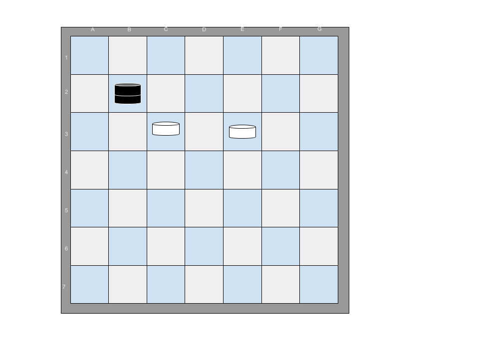
Checkerboard 1 - demonstrate solution

If an additional white piece is added, there is no sequence of moves that will allow any black piece to jump all of the white pieces.
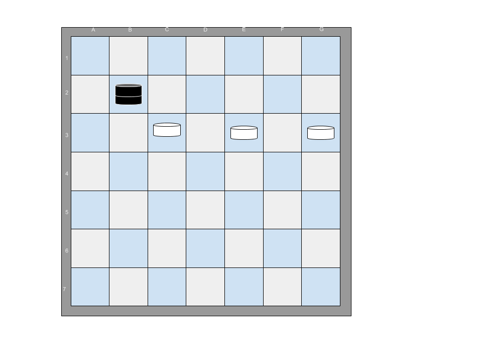
Checkerboard 2 - demonstrate no solution

Input File

The input file consists of one line with a single integer, representing the size of the (square) board. Following are characters representing the board state.

. represents a square that pieces cannot occupy - the off-color squares.

_ represents an unoccupied but valid square.

B represents a black piece. W represents a white piece.

Example:

8
._._._._
_._._._.
.W._.B._
_.W.W._.
.W.B._._
_._._._.
.W._.W._
_._._._.

Output

The output is simple: simply state which of the black checkers is capable of jumping each of the white checkers. If none, say "None". If multiple, say "Multiple".

The Solution

Keep It Simple

To successfully solve the checkers problem, it is important to keep it simple. There are different ways of representing the checkers problem abstractly, but the best representation in a program is the simplest one - use a 2D array of chars to represent the board.

Also as usual with permutations of arrangements on boards of fixed size, recursion will be useful here.

Solution Analysis: Parity

We can begin our analysis of the checkers problem with a few observations.

First, we know that the valid squares for checkers are squares that are off by two. But we know further that the black checkers must only move in jumps, which mean that a piece at \((i,j)\) can only reach squares indexed by \((i + 4m, j + 4m)\) or \((i + 4m + 2, j + 4n + 2)\), where \(m, n\) are positive/negative integers.

That is, the checker pieces can make jumps of 2 squares at a time. For example, if a checker starts at the square \((3,3)\) and jumps a white piece down and to the right, it moves to square \((5,5)\) or \((3+2, 3+2)\). If it jumps another white piece up and to the right, it moves to square \((3, 7)\) or \((3, 3 + 4)\).

Further, we know that a black checker can only jump checkers at squares of the form \((a + 2m + 1, b + 2n + 1)\). Thus, black checkers either have the correct parity to jump all of the white checkers, or they have the same parity as the white checkers (in which case they can be ignored).

If a black checker does not have the correct parity to jump white checkers, we can save ourselves time by not checking it.

For example, in the checkerboard below, there are four black checkers, but only one (row 2, column 3) has the correct parity to jump each of the white pieces. The other three are

The other three has the correct parity, while the black checker in the right do not.
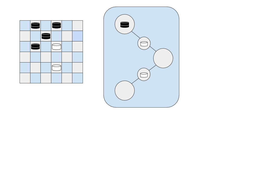
Checkerboard 3 - illustrate parity

Solution Analysis: Graphs and Euler Tours

If we examine the squares with correct parity, we can translate the board into a graph representation. Squares with the "jump" parity are nodes on the graph that can perform jumps. (No whites should have jump parity, otherwise the board is impossible.)

Squares with the "jumped" (i.e., white pieces) parity are nodes that are being jumped. These nodes form the edges between jump parity nodes, and these edges must be occupied by a white piece for a black piece to be able to pass through them. In this way, we can think of white pieces as "bridges" between jump parity squares.

This representation leads to thinking about the tour the black checker takes through the checkerboard as an Euler tour across the graph.

An Euler Tour, made famous by the Seven Bridges of Königsberg problem solved by Euler in 1736, is a path that visits each node of the graph, traversing each edge once and only once.

Euler showed that an Euler path visiting each edge of the graph depends on the degree of each node in the graph. For an Euler path to exist, the graph must be connected and there must be exactly zero or two nodes of odd degree.

If we walk through the checker board and construct the graph (or assemble the information that the graph would have told us), we can determine whether an Euler tour exists, and find the Euler tour.

The example above shows a checkerboard with two white pieces forming two edges. The first white piece connects a jump parity square with a black piece on it to a jump parity square that is empty. The second white piece connects two empty jump parity squares.

The black "entrance" node has an odd degree (1). The second, unoccupied node has an even degree (2). The third, unoccupied node has an odd degree (1). Therefore the graph has two nodes of odd degree, so an Euler tour exists.

If we modify this example to add one additional white checker piece on a square with correct parity, the Euler Path analysis identifies this as a board with no solution:
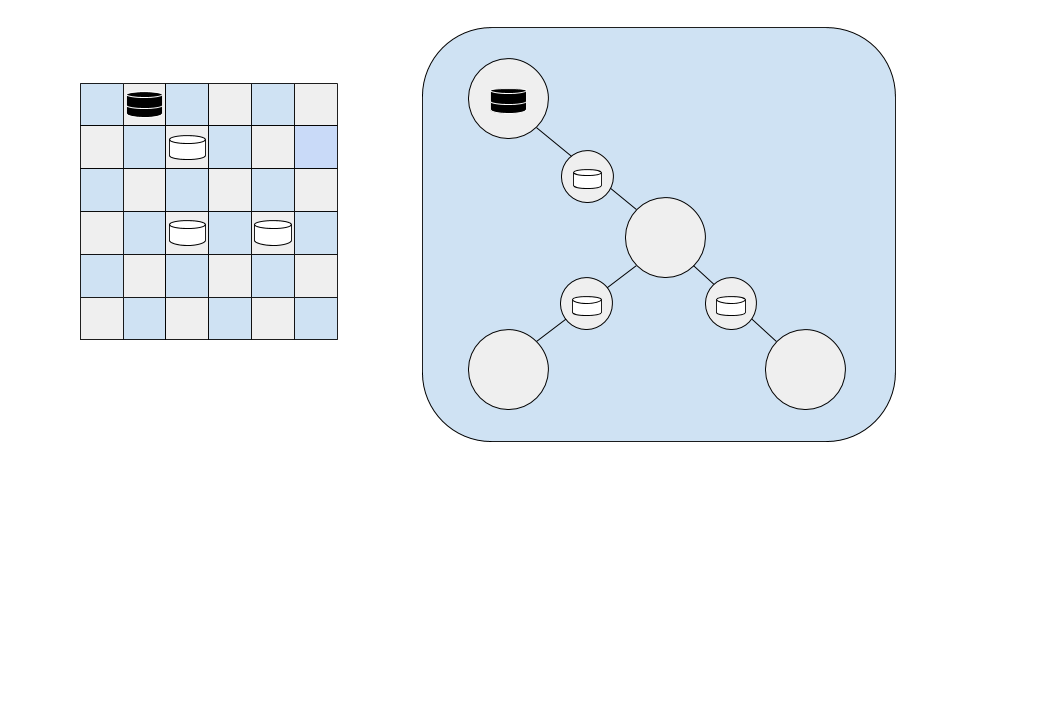
Checkerboard 4 - illustrate no Euler tour

This is because three of the nodes have degree 1 and one node has degree 3, for a total of 4 nodes with odd degree. The requirements for an Euler Tour to exist (equivalent to saying a solution to the Checkers problem can be found for a given black checker) are violated, so no solution can be found.

If we were to add a second black checker piece two squares away, an alternate graph (highlighted in blue) can be constructed, and an alternate Euler path through the graph is available.
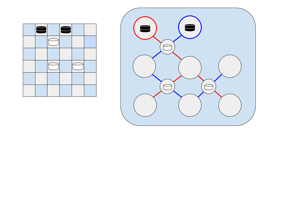
Checkerboard 5 - illustrate alternate Euler tour

On the red graph, each node has an odd degree, so the number of nodes with odd degree is not 0 or 2. On the blue graph, only the start and end nodes have an odd degree (1), while the rest of the nodes have a degree of 2 (one input and one output). This means an Euler Tour exists on the blue graph.

In practice, a given black piece has a given graph connecting squares on the checkerboard - we can ask each node on that graph for its degree, and the degree of its neighbors, and if a black piece results in an invalid number of odd nodes, we can abandon it.

Solution Algorithm

The algorithm to find solutions to this problem very roughly follows this pattern: * First, perform a parity check to determine if a solution is impossible. * Loop over each square of the board, looking for black pieces * For each black piece: * Look at each neighbor: * Determine if there is a square to jump to if neighbor is white * Determine number of odd neighbors * Fail if more than 2 odd neighbors, or 2 odd neighbors and odd self * Backtracking: explore neighbors, determine if all whites can be jumped

Solution Pseudocode

The solution code has three basic parts (four, including the input parser): * Initialize and parse the board * Loop over each square, checking if black piece is a solution * Function to check if black piece is a solution piece * (Recursive backtracking) function to jump each white piece possible to jump.

Start with the initialization of the board and looping over each black piece to check if it is a solution piece:

initialize solutions counter
initialize board

for each s in squares:
    if s is black piece:
        if s is solution piece:
            increment solutions counter
            save location

print summary

Now we just need to implement functions that can (a) check if a square contains a black piece (easy) and (b) check if a black piece is a solution piece (uh... kind of what the whole problem boils down to, no?)

We break that functionality into a separate function. Here is the pseudocode to check if a black piece in a particular square is a solution piece. This function iterates over squares with jump parity - that means this function traverses the nodes only in the graph representation of the checkerboard.

This function enforces the requirement that no node can have more than 2 odd neighbors, or be odd if it has more than 2 odd neighbors, since a graph must have 0 or 2 nodes with odd degree in the graph for an Euler Tour to exist.

While we're at it, we also check if there are any white checker pieces without a square to land in when they are jumped (i.e., landing square blocked by another black piece or at edge of board).

function is solution piece:
    for each square of similar "jump" parity:
        for each neighbor:
            check if neighbor is odd 
            if a neighbor square is white:
                if next square is not empty:
                    fail fast

    if more than 2 odd neighbors, or 2 neighbors and odd:
        fail fast

    # we have a viable solution

    recursively count number of jumped white checkers 

    if number of jumped white checkers equals number of white checkers on board:
        return true

Finding squares of similar jump parity is as easy as looping over each row and column, and checking if it is off by 2 with the row/column of the black checker piece that we are currently checking. Checking if a neighbor is odd is as straightforward as counting its degree - checking each of its four neighbors and determining which ones are open. This leaves finding the number of jumped white checkers as the only functionality left to define.

define number of jumped white checkers:
    initialize white checkers jumped counter
    for each neighbor:
        if white piece, unvisited, with an empty place to jump to:
            visit white piece
            increment white checkers jumped
            call number of jumped white checkers on next next neighbor
            # this should be the empty space
    return number white checkers jumped

References

  1. "ACM Pacific Region Programming Competition." Association of Computing Machinery. 19 June 2017. <http://acmicpc-pacnw.org/>
Teaching Recursion with the N Queens Problem

Posted in Computer Science

permalink

Table of Contents:

A Gentle Introduction to Recursion

Recursion, particularly recursive backtracking, is far and away the most challenging topic I cover when I teach the CSE 143 (Java Programming II) course at South Seattle College. Teaching the concept of recursion, on its own, is challenging: the concept is a hard one to encounter in everyday life, making it unfamiliar, and that creates a lot of friction when students try to understand how to apply recursion.

The key, as I tell students from day one of the recursion unit, is to always think in terms of the base case and the recursive case. The base case gives your brain a "trapdoor" to exit out of an otherwise brain-bending infinite conceptual loop. It helps recursion feel more manageable. But most importantly: it enables thinking about recursion in terms of its inputs and outputs.

More specifically, to understand recursion requires (no, not recursion) thinking about two things: where you enter the function and when you stop calling the function. These are the two least complicated cases, and they also happen to be the two most important cases.

College courses move at an artificially inflated pace, ill-suited for most community college students, and the material prescribed must be presented at the given pace mostly independent of any real difficulties the students face (there is only minimal room for adjustment, at most 2-3 lectures).

This means that, before the students have had an opportunity to get comfortable with the concept of recursion, and really nail it down, they're introduced to yet another mind-bending topic: recursive backtracking algorithms.

These bring a whole new set of complications to the table. Practice is crucial to students' understanding, and all too often, the only way to get students to practice (particularly with difficult subject matter like recursion) is to spend substantial amounts of time in class. My recursion lectures routinely throw my schedule off by nearly a week, because even the simplest recursion or backtracking exercise can eat up an hour or more.

Recursive Backtracking

Backtracking is an approach for exploring problems that involve making choices from a set of possible choices. A classic example of backtracking is the 8 Queens problem, which asks: "How many ways are there of placing 8 queens on a chessboard, such that no queen attacks any other queen?"

The problem is deceptively simple; solving it requires some mental gymnastics. (By the way, most people who have actually heard of the problem are computer scientists who were exposed to it in the process of learning how to solve it, leading to the hipster effect - it's often dismissed by computer scientists as an "easy" problem. The curse of knowledge at work.)

The recursive backtracking algorithm requires thinking about the squares on which to place the 8 queens in question as the set of choices to be made.

The naive approach ignores the constraints, and makes all 8 choices of where to place the 8 queens before ever checking if the queen placements are valid. Thus, we could start by placing all 8 queens in one single row on the top, or along one single column on the left. Using this approach, we have 64 possibilities (64 open squares) for the first queen, then 63 possibilities for the second queen, then 62 possibilities for the third queen, and so on. This gives a total number of possible combinations of:

$$ \dfrac{64!}{(64-8)!} = 178,462,987,637,760 $$

(By the way, for those of you following along at home, you can do this calculation with Python:)

>>> from scipy import *
>>> math.factorial(64)/math.factorial(64-8)
178462987637760L

Even for someone without a sense of big numbers, like someone in Congress, that's still a pretty big number. Too many for a human being to actually try in a single lifetime.

Paring Down the Decision Tree

But we can do better - we can utilize the fact that the queen, in chess, attacks horizontally and vertically, by doing two things:

  • Limit the placement of queens so that there is one queen per column;

  • Limit the placement of queens so that there is one queen per row.

(Note that this is ignoring diagonal attacks; we'll get there in a minute.)

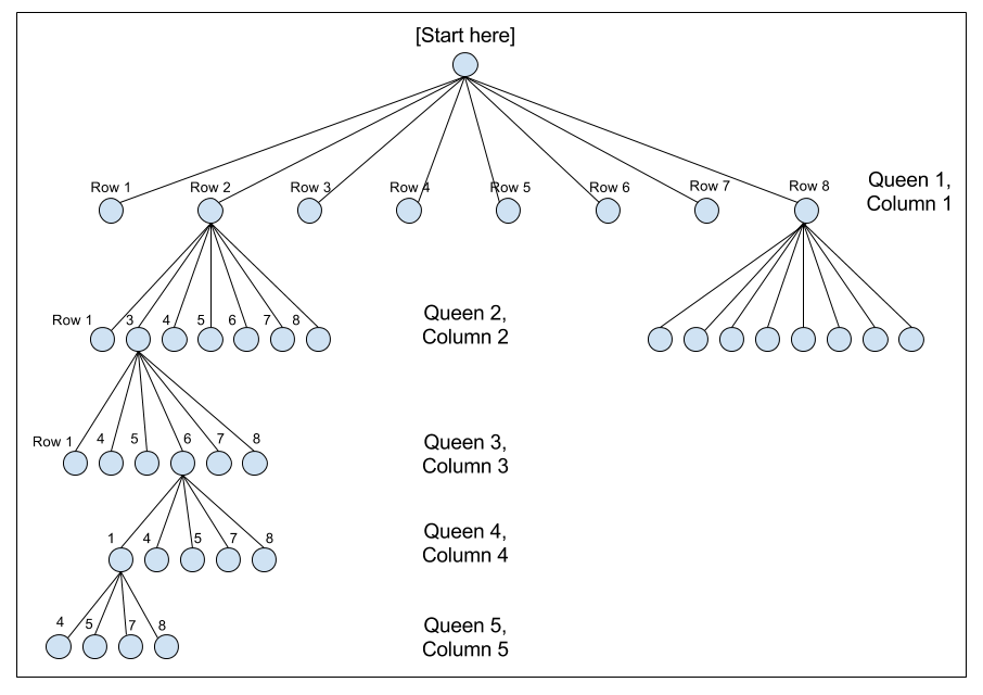
This limits the number of solutions as follows: the first queen placed on the board must go in the first column, and has 8 possible squares in which it can go. The second queen must go in the second column, and has 7 possible squares in which it can go - ignoring the square corresponding to the row that would be attacked by the first queen. The third queen goes into the third column, which has 6 open squares (ignoring the two rows attacked by the two queens already placed).

That leads to far fewer solutions:

$$ 8! = 40,320 $$

and for those following along at home in Python:

>>> from scipy import *
>>> math.factorial(8)
40320

To visualize how this utilization of information helps reduce the problem space, I often make use of a decision tree, to get the students to think about recursive backtracking as a depth-first tree traversal.

(By the way, this is a strategy whose usefulness extends beyond the 8 queens problem, or even recursive backtracking problems. For example, the problem of finding cycles in a directed graph can be re-cast in terms of trees.)

So far, we have used two of the three directions of attack for queens. This is also enough information to begin an implementation of an algorithm - a backtracking algorithm can use the fact that we place one queen per column, and one queen per row, to loop over each row, and steadily march through each column sequentially (or vice-versa).

The Pseudocode

There is still a bit more to do to cut down on the problem space that needs to be explored, but before we do any of that, we should first decide on an approach and sketch out the psuedocode.

The structure of the explore method pseudocode thus looks like:

explore(column):
    if last column:
        # base case
        add to solutions
    else:
        # recursive case
        for each row:
            if this is a safe row:
                place queen on this row
                explore(column+1)
                remove queen from this row

The Actual Code

Over at git.charlesreid1.com/charlesreid1/n-queens I have several implementations of the N Queens problem:

Row, Column, and Diagonal Attacks

We have already utilized knowledge that there will only be one queen per column, and one queen per row. But one last bit of information we can utilize is the fact that queens attack diagonally. This allows us to eliminate any squares that are along the diagonals of queens that have already been placed on the board.

How to eliminate the diagonals? It basically boils down to two approaches:

  1. Use a Board class to abstract away details (and the Board class will implement "magic" like an isValid() method).

  2. Hack the index - implement some index-based math to eliminate any rows that are on the diagonals of queens already on the board.

The first approach lets you abstract away the details, possibly even using a Board class written by a textbook, which is lazy fine, if you are working on a practical problem and need some elbow grease, but not so much if you are a computer science student learning the basic principles of software design.

The second approach requires some deep thinking about how the locations of the N (or 8) queens are being represented in the program.

Accounting for Diagonal Attacks

At some point, when you use the above pseudocode, you are going to want to know the answer to the following question: for a given column k, what rows are invalid because they are on diagonals of already-placed queens?

To answer this, think about where the diagonal indices of chess board squares are located, and how to find the diagonals on column X attacked by a queen placed in column Y.

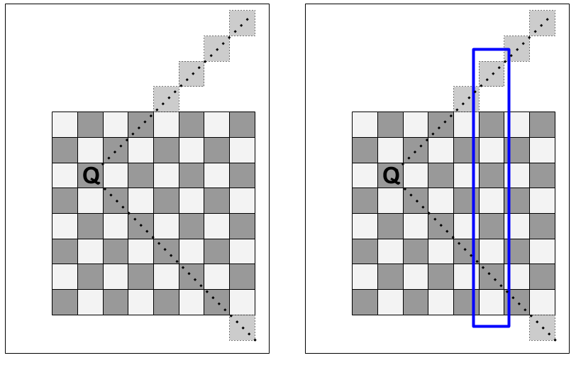
The following diagram shows a queen on row 3 of column 2, and the diagonal attack vectors of that queen. Each of the squares along those diagonal vectors can be ruled out as possible squares to place a queen. When selecting a square for the third queen, which goes in the third column, the second and fourth rows can both be ruled out due to the diagonals. (The third row, of course, can also be ruled out, due to the one-queen-per-row rule.)

However, the effect of the already-placed queen propagates forward, and affects the choice of possible squares for each queen after it. If we jump ahead in the recursive algorithm, to say, queen number 6, being placed on column number 6 (highlighted in blue), the queen in column 2 (row 3) still affects the choice of squares for that column (as do all queens previously placed on the board). In the case pictured in the figure, the seventh row (as well as an off-the-board row) of column 6 can be ruled out as possible squares for the placement of the 6th queen.

Accounting for these diagonal attacks can lead to substantial speed-ups: each queen that is placed can eliminate up to two additional squares per column, which means the overall decision tree for the N queens problem becomes a lot less dense, and faster to explore.

Why the N Queens Problem?

Invariably, some students will deal with this difficult problem by questioning the premise of the question - a reasonable thing to wonder.

This leads to a broader, more important question: why do computer scientists focus so much on games?

Games, like computers, are self-contained universes, they are abstract systems, they remove messy details and complications. They allow you to start, from scratch, by setting up a board, a few rules, a few pieces - things that are easy to implement in a computer.

Mazes, crossword puzzles, card games, checkers, chess, are all systems with a finite, small number of elements that interact in finite, small numbers of ways. The beauty of games is that those small rule sets can result in immensely complex systems, so that there are more branches in the chess decision tree (the Shannon number, \(10^{120}\)) than there are protons in the universe (the Eddington number, \(10^{80}\)).

That simplicity is important in computer science. Any real-world problem is going to have to be broken down, eventually, into pieces, into rules, into a finite representation, so that anything we try to model with a computer, any problem we attempt to solve computationally, no matter how complex, will always have a game-like representation.

(Side note: much of the literature in systems operations research, which studies the application of mathematical optimization to determine the best way to manage resources, came out of work on war games - which were themselves game-ified, simplified representations of real, complex systems. Econometrics, or "computational economics," is another field where game theory has gained much traction and finds many practical applications.)

Recursion, too, is a useful concept in and of itself, one that shows up in sorting and searching algorithms, computational procedures, and even in nature.

But it isn't just knowing where to look - it's knowing what you're looking for in the first place.

Tags:    java    algorithms    recursion    n-queens   

Undergraduate Research Project: Wireless Sensor Networks for Internet of Things Applications (Part 2: The Technologies)

Posted in Wireless

permalink

Undergraduate Research Project (UGR): The Technologies

In this post we'll cover some of the technologies that were used in our South Seatte College undergraduate research project. The project involved an ensemble of different technologies to complete each component of the data analysis pipeline. Some components were planned for, but other components were implemented due to "surprise" challenges that cropped up during the course of the project, while yet more technologies were integrated into the pipeline to avoid extra costs.

Overview of the UGR Project

Before we go further, let's recap what the project was all about. As the research project mentor, I was leading a group of five undergraduate students in a project entitled "Wireless Sensor Networks for Internet of Things Applications." This involved guiding students through the construction of a data analysis pipeline that would utilize a set of sensors, each collecting data about wireless networks in the vicinity, and collect the data into a central database. We then impemented data analysis and visualization tools to analyze the sensor data that was collected and extract meaningful information from it.

There were three major sets of tools used - those used onboard the Raspberry Pi sensors (to extract and transfer wireless data), those used to store and organize the wireless sensor data (NoSQL database tools), and those used to process, analyze, and visualize the data colleted (Python data analysis tools).

The technologies used can be classified two ways:

  • Student-Led Components - the software components of the pipeline that students learned about, and whose implementation was student-led.

  • Backend Components - the software components of the pipeline that were too complicated, too hairy, and/or too extraneous to the project objectives to have students try and handle. These were the components of the project that "just worked" for the students.

Student-Led Components

Raspberry Pi

The Raspberry Pi component presented some unique challenges, with the chief being, enabling the students to actually remotely connect via SSH to a headless Raspberry Pi.

This deceptively simple task requires an intermediate knowledge of computer networking, and coupled with the obstreperous Raspberry Pi, a restrictive college network, the additional complications of students running Linux via virtual machines on Windows (all of the students were using Windows)... It ended up taking more than a month to be able to consistently boot up the Pi, remotely SSH to the Pi, and get a command line using either a crossover cable or a wireless network.

Part of this was induced by hardware, but part was due to unfamiliarity with SSH and Linux, the problems that constantly cropped up ("X is not working in the virtual machine") that were trivial for me to solve, but enigmas for the students, who often did not possess Google-fu.

Question Skills

This last point is subtle but important: the simple skill of knowing what questions to ask, and how to ask them, be they questions asked of a machine or a person or a data set, was one of the most important skills the students gained during this process. These skills go beyond the usual computer science curriculum, which consists of learning structured information in terms of languages and functionality, and require students to solve unstructured problems that are complex - so complex, they simply do not care about languages or functionality.

The flexibility to use many tools was a key element of this project, and a principal reason to use a scripting language (Python) that was flexible enough to handle the many tasks we would be asking of it.

A word about networking issues that the students had connecting to the headless Raspberry Pis:

  • Issues were due to a combination of hardware and networking problems

  • Many issues required multi-step workarounds

  • Workarounds introduced new concepts (DHCP, subnets, IP configuration schemes, IPv6)

  • Each new concept introduced led students to feel overwhelmed

  • Students had a difficult time telling what steps were "normal" and which were esoteric

  • There is a lot of documentation to read - especially difficult for non-English speakers

Each of the multitude of problems students experienced arose from different aspects of the machines. Each problem (networking, hardware, physical power, cables, networking, packet dropping, interfaces, incorrect configuration, firewalls) led to more concepts, more software, more commands.

It can be difficult to troubleshoot networking and hardware issues. It is even more difficult to explain the problem while you are troubleshooting it, and also explain things are important and that students should learn more about, versus some concept that is of questionable usefulness. (Case in point: regular expressions.) On top of that, it is difficult to constantly make judgment calls about what things are important, how important they are, and also helping students not to feel overwhelmed by all the things they don't know yet.

All the while, you are also teaching Google-fu. Did I mention that many of the students do not speak English as their first language?

Aircrack/Airodump

Once the students had reached the Raspberry Pi command line, we moved on to our next major tool - the aircrack-ng suite. This was a relatively easy tool to get working, as it was already available through a package manager (yet another new concept for the students), so we did not waste much time getting aircrack operational and gathering our first sensor data. However, to interpret the output of the tool required spending substantial time covering many aspects of networking - not just wireless networks, but general concepts like packets, MAC addresses, IP addresses, DHCP, ARP, encryption, and the 802.11 protocol specification.

Initially I had thought to use a Python library called Scapy, which provides functionality for interacting with wireless cards and wireless packets directly from Python. My bright idea was to use aircrack to show students what kind of information about wireless networks can be extracted, and to write a custom Python script that would extract only the information we were interested in.

Unfortunately, the complexity of Scapy, and the advanced level of knowledge required of users (even to follow the documentation), meant the tool overwhelmed the students. We wound up practicing putting wireless USB devices into monitor mode from the command line, and starting the wireless network signal profiling tool.

The approach we adopted was to collect wireless network data using aircrack-ng's airodump-ng tool, and to dump the network data at short intervals (15 seconds) to CSV files. These CSV files were then post-processed with Python to extract information and populate the database.

By the end of the first quarter of the project, we were able to utilize airodump-ng to collect wireless network data into CSV files, and parse the data with a Python script.

Pi CSV Files

Further complicating the process of collecting wireless network data from Raspberry Pis was the fact that we were gathering data from the Pis in a variety of different environments - most of which were unfamiliar, and would not reliably have open wireless networks or networks that the Pi was authorized to connect to. Even on the South Seattle campus, the network was locked down, with only HTTP, HTTPS, and DNS traffic allowed on ports 80, 443, and 53, respectively.

This meant we couldn't rely on the Pis making a direct connection to the remote server holding the central database.

Instead, we utilized rsync to synchronize the CSV files gathered by the Pi with the remote server, and we offloaded the process of extracting and analyzing data from the CSV files to a script on the remote server.

That way, the Pis gather the raw data and shuttle the raw data to the remote server (whenever it is available), and the data extraction and analysis process can be performed on the raw data in the CSV files as many times as necessary. If the analysis required different data, or needed to be re-run, the process could simply be updated and re-run on the databae server, with the Raspberry Pi removed from the loop.

NoSQL Database

We needed a warehouse to store the data that the Raspberry Pis were gathering. The aircrack script was dumping CSV files to disk every 15 seconds. Rather than process the data on-board the Raspberry Pi, the script to extract and process data from the CSV files was run on the computer running the database.

This is a best practice I learned form experience:

  • Extract and process the sensor data on-premises (i.e., near or where the data is stored)

  • Keep the original, raw data whenever possible, transport it to the data storage

  • Assume the components of your pipeline will be unreliable or asychronously available

  • Build the pipeline to be robust and handle failures.

We used a cheap, $5/month virtual private server from Linode to run the database. The database technology we chose was MongoDB, mainly because it is a ubiquitous, open-source, network-capable NoSQL database. The NoSQL option was chosen to give students flexibility in structuring the database, and avoid the extra pain of making a weakly-typed language like Python talk to a strongly-typed database system like SQLite or PostgreSQL (which would raise so many questions from students about what is "normal" or "not normal" that I would start to feel like the parent of a bunch of teenagers).

Think of the long-term influence that research mentors can have: simply by showing students how to use vim, and not emacs, I have set them on the path to enlightenment.

We ran the database on the server, but conceptualizing the database was difficult for the students. To this end, I set up an instance of Mongo Express, which provided a password-protected, web-based interface for administering MongoDB that enabled the students to deal with and visualize information more easily.

MongoDB also provided Python bindings via PyMongo, and it was all available for students to install on their local virtual machines and experiment with basic database operations. The MongoDB documentation provides some good examples.

The main struggle that students had was transferring what they had learned about wireless signals and aircrack to the database. Knowing what questions to ask the database proved to take most of their time.

Backend components

During the process of getting each component working, the project occasionally encountered difficulties. The chiefest among these was the fact that the wireless network at our college allowed traffic only on ports 80, 443, and 53, meaning SSH, Rsync, and MongoDB traffic would not make it past the school's firewall.

Stunnel

I have written about Stunnel before on this blog, and have some notes on Stunnel on the charlesreid1.com wiki. This tool proved invaluable for overcoming some of the difficulties on the back-end for the Raspberry Pis.

To allow the Raspberry Pis to securely send data to the database server, I wrote a script that would run on boot and would look for a list of trusted wireless networks, connect to them, and establish an stunnel connection with the remote database server. The script then used rsync over stunnel to synchronize any raw data collected by the Raspberry Pi with the remote database server.

This also satisfied the criteria that the data pipeline be robust and capable of handling failure - this system used stunnel to punch out of a restrictive firewall, and rsync handled comparisons of raw data on the remote and local ends to ensure that only the minimum possible amount of data was transferred between the two. The raw data was plain text and consisted of text files of modest size, making the job easy for rsync.

This was implemented in a boot script, so one simply connected one of the Raspberry Pis to a portable power source (battery pack), and the Pi would look for networks that it trusted, join those networks, and make an stunnel connection over the network to transfer its data (CSV files) to the database server.

Virtual Private Server

Another bit of infrastructure that was provided on the back end was the virtual private server from Linode, so that the students did not have to find a workaround to SSH out of the school's restrictive firewall. A domain for the server was also purchased/provided.

Docker

The virtual private server ran each service in a Docker container - stunnel, MongoDB, MongoExpress, and the long list of Python tools needed to run the Jupyter notebooks for data analysis.

Each Docker container exposed a particular port, making it accessible at an appropriate scope, and by connecting containers to other containers, each component could also seamlessly communicate. Thus one Docker container ran the MongoDB, while another container ran MongoExpress, which established a connection to the MongoDB container.

Using Docker was not strictly necessary, but it was a good opportunity to learn about Docker and get it set up to help solve real-world infrastructure and service problems.

Technologies Flowchart

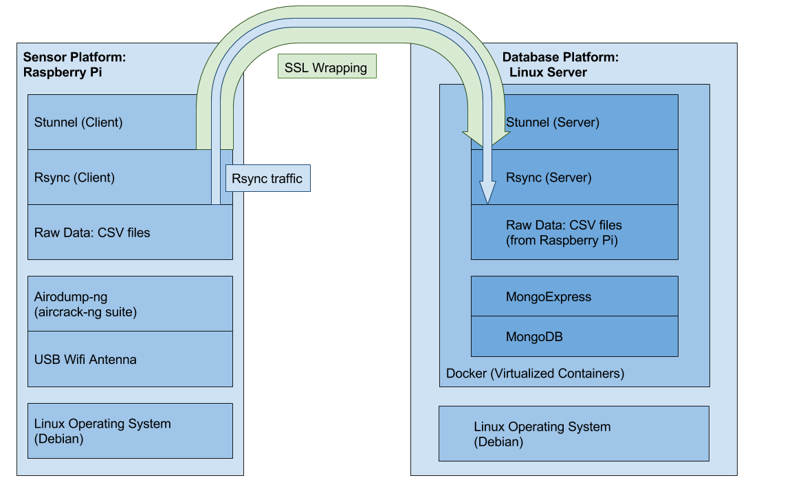
The following flowchart shows the technology stack that was used to coordinate the various moving parts between the Raspberry Pi clients and the remote database server.

UGR Wifi Schematic

Tags:    wireless    security    undergraduate research project    stunnel    SSH    aircrack    mongodb    python    jupyter    linux    raspberry pi   

March 2022

How to Read Ulysses

July 2020

Applied Gitflow

September 2019

Mocking AWS in Unit Tests

May 2018

Current Projects