charlesreid1.com blog

Python vs. Perl: N Queens Problem

Posted in Computer Science

permalink

Table of Contents

Background

Revisiting the N queens problem, this time implementing the solution in Python.

Verb-oriented solution, functional, and based on Perl solution

More fair comparison - both are interpreted languages, not compiled languages

Compare Python and Perl, ease of implementation, speed, flexibility

N Queens Problem

As a recap from the last post about the N queens problem, we're solving a chess puzzle that asks: how many different configurations are there for placing \(N\) queens on an \(N \times N\) chessboard such that no queen attacks any other queen?

This is a popular problem in computer science because solutions often implement recursive backtracking.

See the Wikipedia article for details.

N Queens Solution

Here is the pseudocode of the N queens solution being implemented here:

explore(column):
    if last column:
        # base case
        add to solutions
    else:
        # recursive case
        for each row:
            if this is a safe row:
                place queen on this row
                explore(column+1)
                remove queen from this row

This solution implements recursive backtracking to explore choices of where to place each queen. It keeps solutions simple, and can be implemented using only primitive built-in data types. Solutions are stringified version of these arrays, consisting of 8 digits, so they are likewise very simple.

Perl Solution

As a reminder, the Perl solution was originally from Rosetta Code. Here's another link to the Perl solution on Github.

Github gist: nqueens.pl

Python Solution

The solution requires the use of one array of data that is fixed in size, which for a given column stores a list of rows already occupied by queens, and one array of data that is variable in size, which stores where each queen has been placed.

The Python solution makes use of lists by using a fixed-size list for the occupied rows and a variable size list for storing queen locations. It utilizes buit-in methods for the list data type to append and pop, or add and remove items from the end of the list.

Github gist: nqueens.py

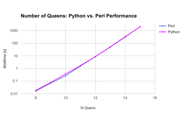
Head to Head: Walltime vs. Number of Queens

Graph of walltime versus number of queens

----------------------------------------------------------
| NQueens | Nsolutions | Java      | Perl     | Python   |
|---------|------------|-----------|----------|----------|
| 8       | 92         | 0.003628  | 0.016    | 0.018    |
| 9       | 352        | 0.006709  | 0.067    | 0.077    |
| 10      | 724        | 0.017473  | 0.259    | 0.359    |
| 11      | 2680       | 0.061291  | 1.542    | 1.684    |
| 12      | 14200      | 0.240463  | 8.431    | 8.618    |
| 13      | 73712      | 1.113491  | 48.542   | 50.401   |
| 14      | 365596     | 6.557336  | 303.278  | 322.576  |
| 15      | 2279184    | 42.619426 | 2057.052 | 1979.343 |
----------------------------------------------------------

The results of this test show that Python and Perl are fairly closely matched.

Perl Profiling

Results of profiling the Perl code with Devel::NYTProf were detailed in a prior post.

Here are those results once again, for the 11 queens problem:

# Profile data generated by Devel::NYTProf::Reader
# Version: v6.04
# More information at http://metacpan.org/release/Devel-NYTProf/
# Format: time,calls,time/call,code
0.000238,2,0.000119,use Time::HiRes qw(time);
0.000039,2,0.000019,use strict;
0.000491,2,0.000246,use warnings;
0.000021,1,0.000021,my $start = time;
0.010338,2680,0.000004,push @solutions, "@queens\n";
0.009993,2680,0.000004,return;
0.186298,164246,0.000001,$#attacked = 2 * $board_size;
0.150338,164246,0.000001,for( 0 .. $#queens) { 
0.675523,1.26035e+06,0.000001,$attacked[ $ix2 ] = 1;
1.242624,164246,0.000008,for my $row (0 .. $board_size-1) {
0.267469,166925,0.000002,explore($depth+1);
0.125272,166925,0.000001,$occupied[$row] = 0;
0.000002,1,0.000002,explore(0);
0.000011,1,0.000011,my $duration = time - $start;
0.000075,1,0.000075,print "Found ", scalar(@solutions), " solutions\n";
0.000050,1,0.000050,printf "Execution time: %0.3f s \n",$duration;

Python Profiling

The Python N queens solution was profiled with two tools: cProfile and line_profiler.

The built-in profiling tool cProfile gives a summary of how much time was spent in each method, but nothing lower level than that. It is similar to Java profiling tools. (cProfile documentation)

The line_profiler tool is designed to profile Python code line-by-line, which gives a much more useful breakdown of where the code spent all of its time. It is also helpful because this can be compared one-to-one with the results from Perl, and we can get an equal basis for comparing the two languages.

Python Profiling Results

cProfile Results

Here are the results from running the N queens problem for N = 11 through cProfile:

**************************************
Profiling 11 queens problem with Python...
*******************************
cProfile:
*******************************
Found 2680 solutions
         996197 function calls (829272 primitive calls) in 2.237 seconds

   Ordered by: internal time

   ncalls  tottime  percall  cumtime  percall filename:lineno(function)
 166926/1    1.845    0.000    2.237    2.237 /Volumes/noospace/Users/charles/codes/hello-world/python/nqueens/nqueens.py:12(explore)
   328492    0.275    0.000    0.275    0.000 {range}
   166925    0.062    0.000    0.062    0.000 {method 'pop' of 'list' objects}
   169605    0.029    0.000    0.029    0.000 {method 'append' of 'list' objects}
   164247    0.026    0.000    0.026    0.000 {len}
        1    0.000    0.000    2.237    2.237 /Volumes/noospace/Users/charles/codes/hello-world/python/nqueens/nqueens.py:4(<module>)
        1    0.000    0.000    0.000    0.000 {method 'disable' of '_lsprof.Profiler' objects}

line_profiler Results

The line_profiler tool gives a more detailed picture of the code and where it spends its time, breaking down profiling information line-by-line. This tool can be installed with pip: pip install line_profiler. The (INSERT LINK)(nqueens repository on github) has a file that demonstrates how to use this tool. See Python/Profiling

Here are the results from the line_profiler tool run on the same (11 queens) problem:

**************************************
Profiling 11 queens problem with Python...
Found 2680 solutions
Wrote profile results to nqueens.py.lprof
Timer unit: 1e-06 s

Total time: 14.2258 s
File: nqueens.py
Function: explore at line 11

Line #      Hits         Time  Per Hit   % Time  Line Contents
==============================================================
    11                                           @profile
    12                                           def explore(depth):
    13                                               # base case
    14    166926       187573      1.1      1.3      if(depth==board_size):
    15                                                   # stringify/serialize the solution
    16      2680        31497     11.8      0.2          solutions.append("%s"%(queens))
    17      2680         3117      1.2      0.0          return
    18                                           
    19                                               else:
    20    164246       384688      2.3      2.7          attacked = 2*board_size*[0,]
    21   1424595      1690693      1.2     11.9          for i in range(0,len(queens)):
    22   1260349      1471304      1.2     10.3              ix1 = queens[i] + depth - i
    23   1260349      1405141      1.1      9.9              attacked[ix1] = 1
    24                                           
    25   1260349      1494095      1.2     10.5              ix2 = queens[i] - depth + i
    26   1260349      1392563      1.1      9.8              attacked[ix2] = 1
    27                                           
    28   1970952      2229922      1.1     15.7          for row in range(0,board_size):
    29   1806706      2031139      1.1     14.3              if(occupied[row] or attacked[row]):
    30    379432       374466      1.0      2.6                  continue
    31                                           
    32                                                       # make a choice
    33    166925       241114      1.4      1.7              queens.append(row)
    34    166925       186833      1.1      1.3              occupied[row] = 1
    35                                           
    36                                                       # explore the consequences
    37    166925       610396      3.7      4.3              explore(depth+1)
    38                                           
    39                                                       # unmake the choice
    40    166925       288667      1.7      2.0              queens.pop()
    41    166925       202555      1.2      1.4              occupied[row] = 0

Python vs Perl: Walltime vs. Number of Solutions Tested

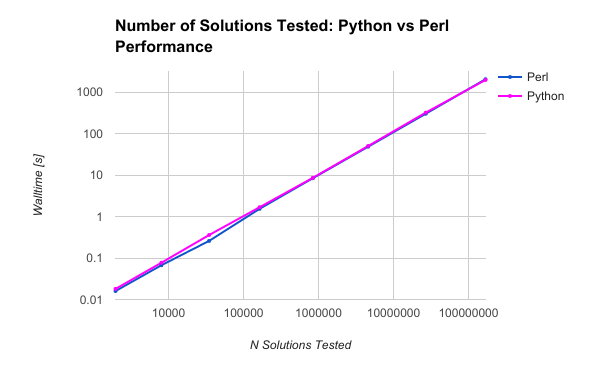
As with the prior post, I verified that both codes were testing the same number of solutions. Here is that table of the number of solutions for each value of N, together with the number of solutions tested:

-----------------------------------------------------------------------------
| NQueens | Nsolutions | NsolutionsTested | Java      | Perl     | Python   |
|---------|------------|------------------|-----------|----------|----------|
| 8       | 92         | 1965             | 0.003628  | 0.016    | 0.018    |
| 9       | 352        | 8042             | 0.006709  | 0.067    | 0.077    |
| 10      | 724        | 34815            | 0.017473  | 0.259    | 0.359    |
| 11      | 2680       | 164246           | 0.061291  | 1.542    | 1.684    |
| 12      | 14200      | 841989           | 0.240463  | 8.431    | 8.618    |
| 13      | 73712      | 4601178          | 1.113491  | 48.542   | 50.401   |
| 14      | 365596     | 26992957         | 6.557336  | 303.278  | 322.576  |
| 15      | 2279184    | 168849888        | 42.619426 | 2057.052 | 1979.343 |
-----------------------------------------------------------------------------

Graph of walltime versus number of solutions tested

The Winner: Perl for Small Problems, Python for Big Ones

It was not a big surprise to see that Perl and Python were nearly identical in their performance, and it testament to the fact that interpreted scripting languages like Perl and Python operate at one speed, and compiled code in C++ or Java operates at a completely different speed that is an order of magnitude faster (see the comparison of Perl and Java in a prior blog post).

Perl and Python were close enough in performance that, although Perl came out ahead on smaller problems and Python came out ahead on the biggest, a different CPU or platform, micro-optimizations, and various butterfly effects could easily turn the tables.

Sources

  1. "N-Queens Problem". Rosetta Code, GNU Free Documentation License. Edited 6 March 2017. Accessed 21 March 2017. <https://web.archive.org/web/20170320081421/http://rosettacode.org/wiki/N-queens_problem>

  2. "nqueens.py". Charles Reid. Github Gist, Github Inc. Edited 25 March 2017. Accessed 25 March 2017. <https://gist.github.com/charlesreid1/1a2ecb3a83284290d4a9daf747d0d7e4>

  3. "nqueens.pl". Charles Reid. Github Gist, Github Inc. Edited 20 March 2017. Accessed 23 March 2017. <https://gist.github.com/charlesreid1/4ce97a5f896ff1c89855a5d038d51535>

  4. "The Python Profilers". Python 2.7.13 Documentation, Python Software Foundation. Updated 20 February 2017. Accessed 23 March 2017. <https://docs.python.org/2/library/profile.html>

  5. "line_profiler". Python Package Index, Python Software Foundation. Updated 20 October 2016. Accessed 23 March 2017. <https://pypi.python.org/pypi/line_profiler/>

  6. "Github - rkern/line_profiler". rkern, Github Repository, Github Inc. Updated 20 October 2016. Accessed 23 March 2017. <https://github.com/rkern/line_profiler>

  7. "Python/Profiling". Charlesreid1.com wiki, Charles Reid. Edited 23 March 2017. Accessed 23 March 2017. <https://web.archive.org/web/20170326031708/http://charlesreid1.com/wiki/Python/Profiling>

Tags:    python    perl    java    algorithms    recursion    n-queens   

Solving the Traveling Salesperson Problem with Java and Guava

Posted in Java

permalink

Table of Contents

Background: Traveling Salesperson Problem (TSP)

The traveling salesperson problem, or TSP, is a classic programming problem and an important one in computer science, and applications in operations research and optimization.

The idea is that you have a set of \(N\) cities, connected by various roads, each with their own distances. That is, we have a set of \(E\) roads, each with their own distance \(d_j, j=1 \dots E\).

The question is, what is the shortest path that a salesperson can take to visit all \(N\) cities, traveling the shortest possible total distance and visiting each city once and only once?

Like the N queens problem, the traveling salesperson problem is a good candidate for recursive backtracking. Also like the N queens problem, there are certain shortcuts we can take to trim down the possibilities we explore.

Computer science pages on Wikipedia are generally pretty high in quality, and the traveling salesman problem page is no exception. It give a very thorough overview of the important aspects of the problem.

Graphs

Graphs are mathematical objects first utilized by Leonhard Euler to solve the Seven Bridges of Köningsberg problem. The concept is simple: you have a bunch of dots connected with lines.

The dots are called nodes, and the lines are called edges.

Graphs can be directed, meaning the edges are like arrows with particular directions, or undirected, meaning the edges simply represent a connection between the two nodes.

Here is an example of a graph with five nodes, with each edge labeled with its distance:
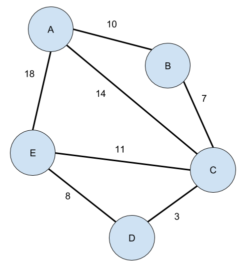
A basic graph with five nodes

We will skip over a vast amount of detail about graph theory that is both fascinating and useful, but M. E. J. Newman's paper "The structure and function of complex networks" (self-published and written as a course review) is an extremely detailed and academically rigorous overview of just about every important detail of the field.

Number of Edges

The maximum number of roads or edges \(E\) depends on the number of nodes as \(E = \dfrac{N(N-1)}{2}\), which is derived from the formula for 2 choose N (because edges connect 2 nodes). For k choose N, the formula is given by:

$$ C_{N,k} = \dfrac{N!}{k! (N-k)!} $$

and for 2 choose N, it is given by:

$$ C_{N,2} = \dfrac{N(N-1)}{2} $$

This is the maximum number of undirected edges in a graph. If the graph is directed, then order matters (the edgge A->B is no longer the same as B->A), so we have to use the formula for k pick N,

$$ P_{N,k} = \dfrac{N!}{(N-k)!} $$

which results in

$$ P_{N,2} = N (N-1) $$

possible edges.

Number of Solutions

Naturally, the question of the total solution space arises. Assuming the graph of cities is perfectly connected (representing an upper limit on problem complexity), how does the number of solutions change as the number of nodes increases?

We can start with a trivial graph, and count the number of possible paths through the entire graph, starting with a specific node. This is equivalent to counting permutations of a string that start with a specific character.

ABCDE
ABCED
ABDCE
ABDEC
ABECD
ABEDC

For a string of length \(N\), the string has \((N-1)!\) possible permutations that start with a specific character. Therefore, as the number of nodes \(N\) increases, the number of possible solutions increases as \((N-1)!\), making the complexity class of the problem \(O(N!)\).

Solution: Recursive Backtracking

Here is pseudocode for a recursive backtracking method:

explore(neighbors):

    if(no more unvisited neighbors):
        # This is the base case.
        if total distance is less than current minimum:
            save path and new minimum

    else:
        # This is the recursive case.
        for neighbor in unvisited neighbors:
            visit neighbor
            explore(new_neighbors)
            unvisit neighbor

Care is needed to prevent infinite loops in which the traveling salesperson goes back and forth between two cities. As we traverse the graph, we can mark each node as visited, to ensure we don't revisit nodes and go in circles.

Nodes can be implemented as a Node object in Java, with each Node having a few characteristics:

  • String label
  • Container of Node pointers pointing to neighbors
  • Boolean flag: have we visited this node already?

Likewise, the graph edges can be represented using integers or doubles.

Solving the TSP with Java and Guava

Google Guava is a library of high-performance data containers in Java. The library provides some useful graph objects that we can use to easily solve the TSP on a graph.

Basics of Guava

Install and use Guava by visiting the Guava project on Github, find the page for their latest release (here is version 21.0), and getting the latest .jar file.

To compile with the jar file, you can either utilize an IDE like Eclipse or IntelliJ, or you can compile from the command line, specifying the class path using the -cp flag:

$ javac -cp '.:/path/to/guava/jars/guava-21.0.jar' TSP.java
$ java -cp '.:/path/to/guava/jars/guava-21.0.jar' TSP

More information can be found on the charlesreid1.com wiki: Guava

Guava Graphs

Graph objects in Guava are implemented using a set of objects: Graphs, ValueGraphs, and Networks.

Graph objects treat edges as very simple and assumes they contain no information and simply link nodes.

ValueGraphs associate a single non-unique value with each edge on the graph. This can also be used to solve the TSP.

Network objects treat nodes and edges both as objects, and has the ability to deal with more complex edges: model multi-edges, repeated edges, directed edges, etc.

We will use a Network object and design our own graph Node and Edge objects.

Link to Guava wiki on how to build graph instances

Guava API Documentation: Network

Guava API Documentation: Graph

Guava API Documentation: ValueGraph

Guava Mutable vs Immutable

Guava makes a distinction between mutable graphs, which can be modified, and immutable graphs, which cannot. Immutability provides some safety and assurances to programmers, and can make things faster.

When we construct the network, we need a mutable graph to modify (add nodes and edges). But once the network is constructed, it is finished: we don't need to modify the network while we're solving the problem.

Therefore, we construct a mutable network, assemble the graph for the given problem, and copy it into an immutable graph. We then use the immutable graph to access the graph while solving.

Importing Guava

Starting with import statements, we'll use a couple of objects from the Java API, and from Google's Guava library:

import java.util.Set;
import java.util.Map;
import java.util.TreeMap;
import java.util.Arrays;

import com.google.common.graph.Network;
import com.google.common.graph.NetworkBuilder;
import com.google.common.graph.ImmutableNetwork;
import com.google.common.graph.MutableNetwork;

For more info on why we don't just do the lazier

import java.util.*;
import com.google.common.graph.*;

see Google's Java style guide.

TSP Class

Let's lay out the TSP class definition. This class is simple, and wraps a few pieces of data: the current route, the current distance, and the minimum distance. Note that we could also save the solution in a container, instead of printing it, by defining a static class to hold solutions, but we'll keep it simple.

/** This class solves the traveling salesman problem on a graph. */
class TSP {
    // The actual graph of cities
    ImmutableNetwork<Node,Edge> graph;
    int graphSize;

    // Storage variables used when searching for a solution 
    String[] route;         // store the route
    double this_distance;   // store the total distance
    double min_distance;    // store the shortest path found so far

    /** Defaut constructor generates the graph and initializes storage variables */
    public TSP() {
        // TODO
    }

    /** This method actually constructs the graph. */
    public ImmutableNetwork<Node,Edge> buildGraph() {
        // TODO
    }

    /** Public solve method will call the recursive backtracking method to search for solutions on the graph */
    public void solve() {
        // TODO
    }

    /** Recursive backtracking method: explore possible solutions starting at this node, having made nchoices */
    public void explore(Node node, int nchoices) {
        // TODO
    }

    /** Print out solution */
    public void printSolution() {
        // TODO
    }

    /** Print out failed path */
    public void printFailure() {
        // TODO
    }

Node Class (Cities)

Now we can define the Node class to represent cities on the graph.

class Node {
    public String label;
    public boolean visited; // Helps us to keep track of where we've been on the graph
    public Node(String name){
        this.label = name;
        this.visited = false;
    }
    public void visit(){
        this.visited = true;
    }
    public void unvisit() {
        this.visited = false;
    }
}

Like a lined list node, we want to keep graph nodes simple. Note that Nodes don't need to store information about their neighbors. That's what we'll use Google Guava for!

Edge Class (Roads)

Edge classes are even simpler, wrapping a single integer:

class Edge {
    public int value;
    public String left, right; // For convenience in construction process. Not necessary.
    public Edge(String left, String right, int value) {
        this.left = left;
        this.right = right;
        this.value = value;
    }
}

Note that left and right are used for convenience only during the graph construction process. Like the nodes, the edges don't need to know who their neighbors are, since that's what the Google Guava graph object will take care of.

TSP Constructor and Building the Graph

Constructor

The TSP class constructor should do a few things:

  • Construct a graph, with a given set of cities and distances.
  • Initialize arrays and cumulative variables that will be used by the backtracking method.

The actual graph construction process is put into another function called buildGraph(), so really the constructor just calls a function and then does #2.

    /** Defaut constructor generates the graph and initializes storage variables */
    public TSP() {
        // Build the graph
        this.graph = buildGraph();
        this.graphSize = this.graph.nodes().size();

        // Initialize route variable, shared across recursive method instances
        this.route = new String[this.graphSize];

        // Initialize distance variable, shared across recursive method instances
        this.this_distance = 0.0;
        this.min_distance = -1.0; // negative min means uninitialized
    }

Build Graph Method

Now we actually use Guava's Immutable Network object, which takes two templated types, T1 and T2, which correspond to the node types and the edge types.

We use a NetworkBuilder object to build the Network (an example of the factory template). This returns a MutableNetwork of Node and Edge objects, which we can then connect up using some built-in methods.

Here are some built-in methods available for a MutableNetwork:

    addEdge(node1, node2, edge)
    addNode(node1)
    removeEdge(edge)
    removeNode(node)

Now here is the construction of the graph, using the Google Guava library. There are two loops here: one for cities, and one for edges. In the loop over each city,we create a new node and add it to the graph. To be able to easily retrieve the Nodes we have created, we also store references to the nodes in a map called all_nodes.

When we construct edges, we use the map of all nodes all_nodes to get references to the Node objects that correspond to a label. That way, if an edge connects "A" with "B" at a distance of 24, we can turn "A" and "B" into references to the Node objects A and B.

    /** This method actually constructs the graph. */
    public ImmutableNetwork<Node,Edge> buildGraph() {

        // MutableNetwork is an interface requiring a type for nodes and a type for edges
        MutableNetwork<Node,Edge> roads = NetworkBuilder.undirected().build();

        // Construct Nodes for cities,
        // and add them to a map
        String[] cities = {"A","B","C","D","E"};
        Map<String,Node> all_nodes = new TreeMap<String,Node>();
        for(int i = 0; i<cities.length; i++) {
            // Add nodes to map
            Node node = new Node(cities[i]);
            all_nodes.put(cities[i], node);

            // Add nodes to network
            roads.addNode(node);
        }

        // Construct Edges for roads,
        // and add them to a map
        String[] distances = {"A:B:24","A:C:5","A:D:20","A:E:18","B:C:10","B:D:20","C:D:4","C:E:28","D:E:3"};
        Map<String,Edge> all_edges = new TreeMap<String,Edge>();
        for(int j = 0; j<distances.length; j++) {
            // Parse out (city1):(city2):(distance)
            String[] splitresult = distances[j].split(":");
            String left = splitresult[0];
            String right = splitresult[1];
            String label = left + ":" + right;
            int value = Integer.parseInt(splitresult[2]);

            // Add edges to map
            Edge edge = new Edge(left, right, value);
            all_edges.put(label, edge);

            // Add edges to network
            roads.addEdge(all_nodes.get(edge.left), all_nodes.get(edge.right), edge);
        }

        // Freeze the network
        ImmutableNetwork<Node,Edge> frozen_roads = ImmutableNetwork.copyOf(roads);

        return frozen_roads;
    }

Solving and Exploring with Recursive Backtracking

Solve Method

The structure of some recursive backtracking problems is to create a public and a private interface, with the public interface taking no parameters or a single parameter that the user will know, and the private method taking a parameter specific to the implementation. That's the pattern we use here.

The solve method sets up the problem by picking a starting node (in this case, an arbitrary starting node). It then gets a reference to that node on the graph, and calls the recursive explore() method, which begins the recursive backtracking method.

    /** Public solve method will call the recursive backtracking method to search for solutions on the graph */
    public void solve() {
        /** To solve the traveling salesman problem:
         * Set up the graph, choose a starting node, then call the recursive backtracking method and pass it the starting node.
         */

        // We need to pass a starting node to recursive backtracking method
        Node startNode = null;

        // Grab a node, any node...
        for( Node n : graph.nodes() ) {
            startNode = n;
            break;
        }

        // Visit the first node
        startNode.visit();

        // Add first node to the route
        this.route[0] = startNode.label;

        // Pass the number of choices made
        int nchoices = 1;

        // Recursive backtracking
        explore(startNode, nchoices);
    }

Explore (Backtrack) Method

And now, on to the recursive backtracking method.

The method takes as a parameter which node we are currently on and the number of cities we have visited. As multiple explore methods choose different paths, they pass references to different node objects in the graph, and they pass different values of nchoices.

The methods, when they do not encounter a solution, will choose a next node and call the explore method on it. Each instance of the explore method marks nodes as visited or unvisited on the same shared graph object. This allows instances of the function to share information about their choices with other instances of the function.

All recursive methods must consist of a base case and a recursive case:

Base case: - We've visited as many cities as are on the graph. - Check if this is a new solution (distance less than the current minimum).

Recursive case: - Make a choice (mark node as visited, add city to route). - Explore the consequences (recursive call). - Unmake the choice (mark node as unvisited, remove city from route). - Move on to next choice.

    /** Recursive backtracking method: explore possible solutions starting at this node, having made nchoices */
    public void explore(Node node, int nchoices) {
        /**
         * Solution strategy: recursive backtracking.
         */

        if(nchoices == graphSize) {
            // 
            // BASE CASE
            //
            if(this.this_distance < this.min_distance || this.min_distance < 0) {
                // if this_distance < min_distance, this is our new minimum distance
                // if min_distance < 0, this is our first minimium distance
                this.min_distance = this.this_distance;
                printSolution();
            } else {
                printFailure();
            }

        } else {
            //
            // RECURSIVE CASE
            //  
            Set<Node> neighbors = graph.adjacentNodes(node);
            for(Node neighbor : neighbors) {
                if(neighbor.visited == false) {

                    int distance_btwn;

                    for( Edge edge : graph.edgesConnecting(node, neighbor) ) {
                        distance_btwn = edge.value;
                    }

                    // Make a choice
                    this.route[nchoices] = neighbor.label;
                    neighbor.visit();
                    this.this_distance += distance_btwn;

                    // Explore the consequences
                    explore(neighbor,nchoices+1);

                    // Unmake the choice
                    this.route[nchoices] = null;
                    neighbor.unvisit();
                    this.this_distance -= distance_btwn;
                }
                // Move on to the next choice (continue loop)
            }               
        } // End base/recursive case
    }

Main and Utility Methods

Last but not least, add the method that actually calls the TSP object's solve method, and define what to do when we encounter a new solution. This program just prints out new solutions as they are found, but you could also add them to a map (map routes to distances), or quietly keep track of the shortest path and not print it until the end.

class TSP {
    public static void main(String[] args) { 
        TSP t = new TSP();
        t.solve();
    }

    ...

Additionally, we may want to perform a certain action when we find a new minimum distance. Note that this method may be called multiple times during the solution procedure.

    /** Print out solution */
    public void printSolution() {
        System.out.print("@@@@@@@@@@\tNEW SOLUTION\t");
        System.out.println("Route: "+Arrays.toString(this.route)
                          +"\tDistance: "+this.min_distance);
    }

    /** Do nothing with failed path */
    public void printFailure() {
        // Nope
    }

Program Output

Initial Graph Structure and Solution

In the construction of the graph, we defined our graph as:

String[] distances = {"A:B:24","A:C:5","A:D:20","A:E:18","B:C:10","B:D:20","C:D:4","C:E:28","D:E:3"};

This is the graph that we're solving the TSP problem on. Here are the results when the program is compiled and run:

$ javac -cp '.:/Users/charles/codes/guava/jars/guava-21.0.jar' TSP.java

$ java -cp '.:/Users/charles/codes/guava/jars/guava-21.0.jar' TSP

@@@@@@@@@@  NEW SOLUTION    Route: [A, B, C, D, E]  Distance: 41.0
@@@@@@@@@@  NEW SOLUTION    Route: [A, C, B, D, E]  Distance: 38.0
@@@@@@@@@@  NEW SOLUTION    Route: [A, E, D, C, B]  Distance: 35.0

The answers given were satisfactory and correct, so we moved on to a more advanced graph construction process that utilized a static class to generate random, fully-connected graphs. This also implemented additional functionality to export to Dot format. This static RandomGraph class will be covered in later post.

Here is the resulting output of the random graph generator for a 6-node TSP problem, with the sequence of shortest routes found by the algorithm:

Six-node traveling salesperson problem

java -cp '.:/Users/charles/codes/guava/jars/guava-21.0.jar' TSP 6 
------------------- TSP ----------------------
!!!!!YAY!!!!!!  NEW SOLUTION    Route: [0, 1, 3, 2, 4, 5]   Distance: 291.0
!!!!!YAY!!!!!!  NEW SOLUTION    Route: [0, 1, 3, 5, 4, 2]   Distance: 249.0
!!!!!YAY!!!!!!  NEW SOLUTION    Route: [0, 1, 2, 4, 3, 5]   Distance: 246.0
!!!!!YAY!!!!!!  NEW SOLUTION    Route: [0, 1, 5, 3, 4, 2]   Distance: 203.0
!!!!!YAY!!!!!!  NEW SOLUTION    Route: [0, 3, 5, 1, 4, 2]   Distance: 178.0
!!!!!YAY!!!!!!  NEW SOLUTION    Route: [0, 2, 4, 1, 5, 3]   Distance: 163.0
 Done.

And for 12 nodes, a problem twice that size, here is the graph and corresponding output:

Twelve-node traveling salesperson problem

and the output:

java -cp '.:/Users/charles/codes/guava/jars/guava-21.0.jar' TSP 12 
------------------- TSP Version 2: The Pessimistic Algorithm ----------------------
!!!!!YAY!!!!!!  NEW SOLUTION    Route: [0, 1, 7, 4, 2, 9, 10, 5, 3, 6, 8, 11]   Distance: 585.0
!!!!!YAY!!!!!!  NEW SOLUTION    Route: [0, 1, 7, 4, 2, 9, 10, 5, 3, 8, 11, 6]   Distance: 558.0
!!!!!YAY!!!!!!  NEW SOLUTION    Route: [0, 1, 7, 4, 2, 9, 10, 5, 3, 8, 6, 11]   Distance: 522.0
!!!!!YAY!!!!!!  NEW SOLUTION    Route: [0, 1, 7, 4, 2, 9, 10, 6, 5, 3, 8, 11]   Distance: 499.0
!!!!!YAY!!!!!!  NEW SOLUTION    Route: [0, 1, 7, 4, 2, 9, 10, 11, 8, 6, 5, 3]   Distance: 460.0
!!!!!YAY!!!!!!  NEW SOLUTION    Route: [0, 1, 7, 4, 2, 9, 10, 11, 6, 8, 3, 5]   Distance: 459.0
!!!!!YAY!!!!!!  NEW SOLUTION    Route: [0, 1, 7, 4, 2, 9, 11, 8, 10, 6, 5, 3]   Distance: 449.0
!!!!!YAY!!!!!!  NEW SOLUTION    Route: [0, 1, 7, 4, 2, 9, 11, 10, 6, 8, 3, 5]   Distance: 419.0
!!!!!YAY!!!!!!  NEW SOLUTION    Route: [0, 1, 7, 4, 2, 9, 11, 10, 8, 6, 5, 3]   Distance: 408.0
!!!!!YAY!!!!!!  NEW SOLUTION    Route: [0, 1, 7, 4, 2, 9, 3, 5, 6, 8, 10, 11]   Distance: 402.0
!!!!!YAY!!!!!!  NEW SOLUTION    Route: [0, 1, 7, 4, 2, 3, 9, 11, 10, 8, 6, 5]   Distance: 385.0
!!!!!YAY!!!!!!  NEW SOLUTION    Route: [0, 1, 7, 4, 11, 10, 8, 6, 2, 9, 3, 5]   Distance: 377.0
!!!!!YAY!!!!!!  NEW SOLUTION    Route: [0, 1, 7, 4, 5, 3, 9, 11, 10, 8, 6, 2]   Distance: 374.0
!!!!!YAY!!!!!!  NEW SOLUTION    Route: [0, 1, 7, 4, 5, 6, 8, 10, 11, 9, 3, 2]   Distance: 371.0
!!!!!YAY!!!!!!  NEW SOLUTION    Route: [0, 1, 7, 9, 3, 5, 4, 11, 10, 8, 6, 2]   Distance: 363.0
!!!!!YAY!!!!!!  NEW SOLUTION    Route: [0, 1, 7, 9, 3, 2, 6, 8, 10, 11, 4, 5]   Distance: 352.0
!!!!!YAY!!!!!!  NEW SOLUTION    Route: [0, 1, 7, 3, 5, 4, 11, 9, 2, 6, 8, 10]   Distance: 350.0
!!!!!YAY!!!!!!  NEW SOLUTION    Route: [0, 1, 7, 3, 2, 9, 11, 4, 5, 6, 8, 10]   Distance: 347.0
!!!!!YAY!!!!!!  NEW SOLUTION    Route: [0, 1, 7, 3, 9, 2, 4, 11, 10, 8, 6, 5]   Distance: 345.0
!!!!!YAY!!!!!!  NEW SOLUTION    Route: [0, 1, 7, 3, 9, 2, 6, 8, 10, 11, 4, 5]   Distance: 323.0
!!!!!YAY!!!!!!  NEW SOLUTION    Route: [0, 1, 7, 5, 3, 9, 2, 6, 8, 10, 11, 4]   Distance: 322.0
!!!!!YAY!!!!!!  NEW SOLUTION    Route: [0, 1, 7, 5, 4, 2, 3, 9, 11, 10, 8, 6]   Distance: 316.0
!!!!!YAY!!!!!!  NEW SOLUTION    Route: [0, 1, 7, 5, 4, 2, 6, 8, 10, 11, 9, 3]   Distance: 313.0
!!!!!YAY!!!!!!  NEW SOLUTION    Route: [0, 1, 7, 5, 4, 11, 9, 3, 2, 6, 8, 10]   Distance: 306.0
!!!!!YAY!!!!!!  NEW SOLUTION    Route: [0, 1, 7, 5, 4, 11, 10, 8, 6, 2, 9, 3]   Distance: 302.0
!!!!!YAY!!!!!!  NEW SOLUTION    Route: [0, 1, 10, 11, 4, 5, 7, 3, 9, 2, 6, 8]   Distance: 289.0
!!!!!YAY!!!!!!  NEW SOLUTION    Route: [0, 1, 10, 8, 6, 2, 9, 3, 7, 5, 4, 11]   Distance: 286.0
!!!!!YAY!!!!!!  NEW SOLUTION    Route: [0, 1, 10, 8, 6, 2, 3, 9, 11, 4, 5, 7]   Distance: 283.0
!!!!!YAY!!!!!!  NEW SOLUTION    Route: [0, 1, 8, 6, 10, 11, 4, 2, 9, 3, 7, 5]   Distance: 274.0
!!!!!YAY!!!!!!  NEW SOLUTION    Route: [0, 1, 8, 6, 10, 11, 4, 5, 7, 3, 9, 2]   Distance: 260.0
!!!!!YAY!!!!!!  NEW SOLUTION    Route: [0, 1, 4, 2, 6, 8, 10, 11, 9, 3, 7, 5]   Distance: 259.0
!!!!!YAY!!!!!!  NEW SOLUTION    Route: [0, 1, 4, 11, 10, 8, 6, 5, 7, 3, 9, 2]   Distance: 256.0
!!!!!YAY!!!!!!  NEW SOLUTION    Route: [0, 1, 4, 11, 10, 8, 6, 2, 9, 3, 7, 5]   Distance: 248.0
!!!!!YAY!!!!!!  NEW SOLUTION    Route: [0, 1, 4, 5, 7, 3, 9, 11, 10, 8, 6, 2]   Distance: 245.0
!!!!!YAY!!!!!!  NEW SOLUTION    Route: [0, 7, 5, 4, 1, 8, 6, 10, 11, 9, 3, 2]   Distance: 236.0
 Done.

Note that these random graphs are fully connected - every node connects to every other node. Among the many interesting aspects of the problem, one of them is the impact of connectivity on the solution time.

Another aspect of the problem is the topology of the network, and exploring how a larger number of unconnected nodes, or groups of nodes clustered together but isolated from one another, affect the final solution time and the final route.

But before get to that, we have some other things to work out.

Next Steps: Timing and Profiling

This post described a working implementation of a recursive backtracking solution to the traveling salesperson problem on a graph. This is a naive solution, however, and in the next few posts about the traveling salesperson problem we'll focus on using timing and profiling tools for Java to profile this Guava program, identify bottlenecks, and speed it up. In fact, there is one small tweak we can make to the algorithm covered above that will improve the performance by orders of magnitude. But more on that in a future post.

Sources

  1. "Traveling Salesman Problem". Wikipedia, the Free Encyclopedia. The Wikimedia Foundation. Edited 12 March 2017. Accessed 23 March 2017. <https://en.wikipedia.org/wiki/Travelling_salesman_problem>

  2. "Seven Bridges of Königsberg". Wikipedia, the Free Encyclopedia. The Wikimedia Foundation. Edited 11 March 2017. Accessed 23 March 2017. <https://en.wikipedia.org/wiki/Seven_Bridges_of_K%C3%B6nigsberg>

  3. "The structure and function of complex networks". M. E. J. Newman. <http://www-personal.umich.edu/~mejn/courses/2004/cscs535/review.pdf>

  4. "Google Guava - Github". Alphabet, Inc. Released under the Apache 2.0 License. Accessed 20 March 2017. <https://github.com/google/guava>

  5. "Guava". Charles Reid. Edited 23 March 2017. Accessed 23 March 2017. <https://www.charlesreid1.com/wiki/Guava>

  6. "Graphs Explained". Google Guava Wiki. Accessed 23 March 2017. <https://github.com/google/guava/wiki/GraphsExplained>

  7. "Network". Google Guava API Documentation. Accessed 23 March 2017. <http://google.github.io/guava/releases/snapshot/api/docs/com/google/common/graph/Network.html>

  8. "Graph". Google Guava API Documentation. Accessed 23 March 2017. <http://google.github.io/guava/releases/snapshot/api/docs/com/google/common/graph/Graph.html>

  9. "Value Graph". Google Guava API Documentation. Accessed 23 March 2017. <http://google.github.io/guava/releases/snapshot/api/docs/com/google/common/graph/ValueGraph.html>

  10. "Google Java Style Guide". Alphabet Inc. Accessed 21 March 2017. <https://google.github.io/styleguide/javaguide.html>
Tags:    computer science    guava    graph    TSP   

Perl vs. Java: N Queens Problem

Posted in Computer Science

permalink

Table of Contents

Summary

In this post, we describe an implementation of the N Queens Problem, which is a puzzle related to optimization, combinatorics, and recursive backtracking. The puzzle asks: how many configurations are there for placing 8 queens on a chessboard such that no queen can attack any othr queen?

This problem was implemented in Perl and in Java, the solution results were timed, and the codes were profiled. While Perl is an interpreted language, and is therefore fully expeted to be much slower than Java (which indeed it is), it is still useful to compare the performance between these two codes to gain an appreciation for the advantages and disadvantages to both approaches.

Background: Huh?

Recently I read an (11 year old) article by Steve Yegge entitled "Execution in the Kingdom of Nouns." In it, Steve describes the way that in Java, "Classes are really the only modeling tool Java provides you. So whenever a new idea occurs to you, you have to sculpt it or wrap it or smash at it until it becomes a thing, even if it began life as an action, a process, or any other non-'thing' concept."

The article inspired me to try on this verb-oriented mode of thinking in a more... active way. Prior experiences with OCaml were confusing, and Haskell continues to evade me, so it was easier to dust off old Perl skills than learn enough Haskell or Ocaml to solve N queens problem. Perl was the next-closest verb-oriented "scripting" language.

I was also familiar with the N queens problem, since I'm a programming instructor (I'll let you guess which language), and it seemed like a nice problem for both noun-based and verb-based approaches. But it also meant I had to learn enough Perl to solve the N queens problem.

...or, use the Perl solution to the N queens problem from Rosetta Code.

Right...

So here's the plan: study a verb-oriented implementation of this canonical, deceptively subtle programming problem in Perl; translate it into a verb-oriented Java program; and run the two head-to-head, using a profiler to understand the results.

N Queens Problem

The N queens problem predates computers - it's a chess puzzle that asks: how many ways can you place 8 queens on a chessboard such that no queen can attack any other queen?

The number of possible configurations of queens on a chessboard is 64 pick 8, or

$$ \dfrac{64!}{(64-8)!} = 64 \times 63 \times \dots \times 57 \times 56 = 178,462,987,637,760 $$

Here's that calculation in Python:

>>> import numpy as np
>>> np.prod(range(64-8+1,64+1))
178462987637760

That's bigger than the net worth of most U.S. Presidents!

If we implemented a dumb brute-force solution that tested each of these configurations, we'd be waiting until the heat death of the universe.

Fortunately, as we place queens on the board we can check if it is an invalid placement, and rule out any configurations that would follow from that choice. As long as we are making our choices in an orderly fashion, this enables us to rule out most of the nearly 10 quadrillion possibilities. If we place queens column-by-column and rule out rows where there are already queens, by keeping track of where queens have already been placed, we can reduce the number of possible rows by 1 with each queen placed. The first queen has 8 possible rows where it can be placed, the second queen has 7 possible rows (excluding the row that the first queen was placed on), and so on. The number of possiblities is:

$$ 8! = 8 \times 7 \times \dots \times 2 \times 1 = 40,320 $$

A big improvement! Here's that calculation in Python:

>>> def fact(n):
...     if(n==1):
...         return 1
...     else:
...         return n*fact(n-1)
...
>>> fact(8)
40320

This still-large number of possibilities can be further reduced by using the same procedure, but checking for invalid rows based on the diagonal squares that each already-placed queen attacks. This covers each precondition for a solved board, and allows the base case of the recursive backtracking method to be as simple as, "If you've reached this point, you have a valid solution. Add it to the solutions bucket."

Now, let's get to the solution algorithm.

N Queens Solution

As a recap, we dusted off our Perl skills to utilize an N queens solution in Perl from Rosetta Code.

Here's the pseudocode:

explore(column):
    if last column:
        # base case
        add to solutions
    else:
        # recursive case
        for each row:
            if this is a safe row:
                place queen on this row
                explore(column+1)
                remove queen from this row

Both codes use integer arrays to keep track of where queens are placed. Solutions are stringified version of these arrays, consisting of 8 digits.

Perl Solution

After looking at the Rosetta Code solution for a (long) while and marking it up with comments to understand what it was doing, I decided it was precisely the kind of verb-oriented solution I wanted to test out to compare Perl and Java. It uses no objects, but instead relies on fast built-in data structures (arrays), for loop expansion (only for my $i (1 .. $N), no for($i=1; $i<=$N; $i++)), and basic integer math. The cost of solving the problem comes down to basic indexing and array access.

This is the kind of solution I imagine a human calculator like Alan Turing or John Von Neuman looking at, nodding, and saying, "Makes sense! (And by the way the answer is 92.)"

Github gist: nqueens.pl

#!/usr/bin/perl

# Solve the N queens problem
# using recursive backtracking.
# 
# Author: Charles Reid
# Date: March 2017

# Create an array to store solutions
my @solutions;

# Create an array to store where queens have been placed
my @queens;

# Mark the rows already used (useful for lookup)
my @occupied;

# explore() implements a recursive, depth-first backtracking method
sub explore { 
    # Parameters:
    #   depth : this is the argument passed by the user

    # First argument passed to the function is $depth 
    # (how many queens we've placed on the board),
    # so use shift to pop that out of the parameters 
    my ($depth, @diag) = shift;

    # Explore is a recursive method,
    # so we need a base case and a recursive case.
    #
    # The base case is, we've reached a leaf node,
    # placed 8 queens, and had no problems, 
    # so we found a solution.
    if ($depth==$board_size) { 
        # Here, we store the stringified version of @queens,
        # which are the row numbers of prior queens. 
        # This is a global variable that is shared across
        # instances of this recursive function.
        push @solutions, "@queens\n";
        return;
    }

    # Mark the squares that are attackable, 
    # so that we can cut down on the search space.
    $#diag = 2 * $board_size;
    for( 0 .. $#queens) { 
        $ix1 = $queens[$_] + $depth - $_ ;
        $diag[ $ix1 ] = 1;

        $ix2 = $queens[$_] - $depth + $_ ;
        $diag[ $ix2 ] = 1;
    }

    for my $row (0 .. $board_size-1) {
        # Cut down on the search space:
        # if this square is already occupied
        # or will lead to an invalid solution,
        # don't bother exploring it.
        next if $occupied[$row] || $diag[$row];

        # Make a choice
        push @queens, $row;
        # Mark the square as occupied
        $occupied[$row] = 1;

        # Explore the consequences
        explore($depth+1);

        # Unmake the choice
        pop @queens;

        # Mark the square as unoccupied
        $occupied[$row] = 0;

    }
}

$board_size = 8; 

explore(0);

print "total ", scalar(@solutions), " solutions\n";

Java Solution

Starting with the Rosetta Code solution in Perl, I translated the algorithm into Java, sticking as closely as possible to the Way of the Verb. I replicated the solution in Java with a minimal amount of object-oriented-ness. A Board class simply wraps the same set of arrays and array manipulations that the Perl solution implements directly. These constitute the lookahead check for safe places to put the queen.

The Java solution implements a static class containing a Linked List to store solutions. This is the only use of non-array objects and has a trivial impact on the solution walltime.

Github gist: NQueens.java

(Verbatim code not included for length.)

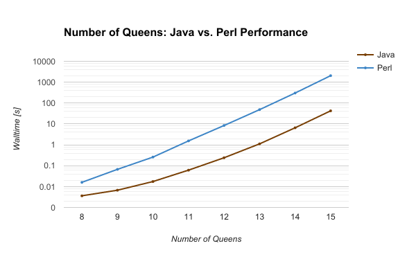
Head to Head: Walltime vs. Number of Queens

Graph of walltime versus number of queens

-----------------------------------------------
| NQueens | Nsolutions | Java [s]  | Perl [s] |
|---------|------------|-----------|----------|
| 8       | 92         | 0.003     | 0.016    |
| 9       | 352        | 0.006     | 0.067    |
| 10      | 724        | 0.017     | 0.259    |
| 11      | 2680       | 0.061     | 1.542    |
| 12      | 14200      | 0.240     | 8.431    |
| 13      | 73712      | 1.113     | 48.542   |
| 14      | 365596     | 6.557     | 303.278  |
| 15      | 2279184    | 42.619    | 2057.052 |
-----------------------------------------------

Java smokes Perl.

Initially I was using the Unix time utility to time these two, and it seemed to be close for smaller problem sizes (N=9 or smaller) - Perl would start up and run faster than Java, measured end-to-end. But when you time the program by using timers built into the language, it removes some of the overhead from the timing comparisons, and Java becomes the clear winner.

We can dig deeper and understand this comparison better by using some profiling tools.

Perl Profiling

I profiled Perl with Devel::NYTProf , an excellent Perl module available here on Cpanm.

More details about the profiling tools I used for Perl are on the charlesreid1 wiki at Perl/Profiling.

To run with Devel::NYTProf, use `cpanm:

$ cpanm Devel::NYTProf

Now you can run Perl with Devel::NYTProf by doing:

$ perl -d:NYTProf nqueens.pl

This results in a binary output file called nytprof.out that can be processed with several NYTProf post-processing tools. Use the CSV file tool to begin with:

$ nytprofcsv nytprof.out

This puts the CSV file in a folder called nytprof/.

Perl Profiling Results

The CSV output of the NYTProf module gives a breakdown of the amount of time spent in each method call, how many times it was called, and how much time per call was spent. From this we can see the busiest lines are the lines accessing the arrays, and looping over the rows. This is confirmation that this algorithm is testing the performance of the arrays, and confirms the N queens problem is profiling Perl's core performance with its built-in data structures.

The profiling results of the 11 queens problem are shown below.

# Profile data generated by Devel::NYTProf::Reader
# Version: v6.04
# More information at http://metacpan.org/release/Devel-NYTProf/
# Format: time,calls,time/call,code
0.000238,2,0.000119,use Time::HiRes qw(time);
0.000039,2,0.000019,use strict;
0.000491,2,0.000246,use warnings;
0.000021,1,0.000021,my $start = time;
0.010338,2680,0.000004,push @solutions, "@queens\n";
0.009993,2680,0.000004,return;
0.186298,164246,0.000001,$#attacked = 2 * $board_size;
0.150338,164246,0.000001,for( 0 .. $#queens) { 
0.675523,1.26035e+06,0.000001,$attacked[ $ix2 ] = 1;
1.242624,164246,0.000008,for my $row (0 .. $board_size-1) {
0.267469,166925,0.000002,explore($depth+1);
0.125272,166925,0.000001,$occupied[$row] = 0;
0.000002,1,0.000002,explore(0);
0.000011,1,0.000011,my $duration = time - $start;
0.000075,1,0.000075,print "Found ", scalar(@solutions), " solutions\n";
0.000050,1,0.000050,printf "Execution time: %0.3f s \n",$duration;

One of the more interesting pieces of information comes from several lines populating the squares that are on the diagonals with other queens ($attacked):

# Format: time,calls,time/call,code
0.186298,164246,0.000001,$#attacked = 2 * $board_size;

The second column gives the number of times this line is executed - 164,246. This is actually the number of solutions that are tried, excluding the deepest depth of the tree (the base recursive case).

The Java profiler will show us that Java explores the exact same number of solutions, which is confirmation that these tests are comparing the two languages on equal footing.

Java Profiling

More details about the profiling tools I used for Java are on the charlesreid1 wiki at Java/Profiling

I profiled Java with two tools, the Java Interactive Profiler (JIP) and the HPROF tool that Oracle provides with Java.

No special compiler flags are needed, so compile as normal:

$ javac NQueens.java

If you are profiling with JIP, you want the JIP jar, as described on the wiki: Java/Profiling Then run Java with the -javaagent flag:

$ export PATH2JIP="${HOME}/Downloads/jip"
$ java -javaagent:${PATH2JIP}/profile/profile.jar NQueens

This results in a profile.txt file with detailed profiling information (an example is shown below).

The HPROF tool likewise requires no special compiler flags. It can be run with various options from the command line. Here's a basic usage of HPROF that will reduce the amount of output slightly, making the size of the output file a little smaller:

$ java -agentlib:hprof=verbose=n NQueens

This dumps out a file called java.hprof.txt that contains a significant amount of information. The most useful, though, is at the end, so use tail to get a quick overview of the results:

$ tail -n 100 java.hprof.txt

Java Profiling Results

The profiling results from JIP for the 11 queens problem are shown below.

+----------------------------------------------------------------------
|  File: profile.txt
|  Date: 2017.03.19 19:34:18 PM
+----------------------------------------------------------------------

+--------------------------------------+
| Most expensive methods summarized    |
+--------------------------------------+

               Net
          ------------
 Count     Time    Pct  Location
 =====     ====    ===  ========
166926    909.5   82.2  NQueens:explore
164246     55.6    5.0  Board:getDiagAttacked
166925     41.4    3.7  Board:unchoose
166925     40.7    3.7  Board:choose
164246     31.0    2.8  Board:getOccupied
     1     18.2    1.6  NQueens:main
  2680      7.3    0.7  Board:toString
  2680      2.3    0.2  SolutionSaver:saveSolution
     1      0.2    0.0  SolutionSaver:nSolutions
     1      0.1    0.0  SolutionSaver:<init>
     1      0.0    0.0  Board:<init>

From this output we can see that the method getDiagAttacked, which is called each time we check a solution in the recursive case, is called 164,246 times - exactly the same number of solutions that the Perl profiler showed. One of the downsides of the JIP profiler is that it only gives high-level profiling information about methods and classes - it stops there.

Fortunately, however, the HPROF tool picks up where JIP leaves off. The HPROF tool makes the program much slower but yields a huge amount of information. In addition to an enormous heap dump of all objects appearing on Java's heap at any point, it also shows where the time was spent in the low-level methods.

SITES BEGIN (ordered by live bytes) Sun Mar 19 19:34:21 2017
          percent          live          alloc'ed  stack class
 rank   self  accum     bytes objs     bytes  objs trace name
    1 86.01% 86.01%  10510976 164234  10510976 164234 300462 int[]
    2  1.93% 87.94%    235840 2680    235840  2680 300467 char[]
    3  1.09% 89.03%    133320 1515    133320  1515 300465 char[]
    4  1.07% 90.11%    131200    8    131200     8 300263 char[]
    5  1.05% 91.16%    128640 2680    128640  2680 300464 char[]
    6  1.04% 92.20%    127560 1313    127560  1313 300010 char[]
    7  0.76% 92.96%     92728 1009     92728  1009 300000 char[]
    8  0.54% 93.50%     65664    8     65664     8 300260 byte[]
    9  0.53% 94.02%     64320 2680     64320  2680 300468 java.util.LinkedList$Node
   10  0.53% 94.55%     64320 2680     64320  2680 300466 java.lang.String
SITES END

HPROF tells us that over 86% of the time spent on this program was spent accessing integer arrays. Again, confirmation that we are getting a fair measurement of Java's performance with a core data type, the integer array.

Head to Head: Walltime vs. Number of Solutions Tested

Using the results of the profilers from each N queens problem, N = 8 .. 15, I extracted the total number of solutions tried, and confirmed that these numbers were the same between Java and Perl for each of the problem sizes.

Here is a table of the number of solutions found, and number of solutions tried, versus problem size:

-------------------------------------------------------------
| NQueens | Nsolutions | Ntested     | Java [s]  | Perl [s] |
|---------|------------|-------------|-----------|----------|
| 8       | 92         | 1965        | 0.003     | 0.016    |
| 9       | 352        | 8042        | 0.006     | 0.067    |
| 10      | 724        | 34815       | 0.017     | 0.259    |
| 11      | 2680       | 164246      | 0.061     | 1.542    |
| 12      | 14200      | 841989      | 0.240     | 8.431    |
| 13      | 73712      | 4601178     | 1.113     | 48.542   |
| 14      | 365596     | 26992957    | 6.557     | 303.278  |
| 15      | 2279184    | 168849888   | 42.619    | 2057.052 |
-------------------------------------------------------------

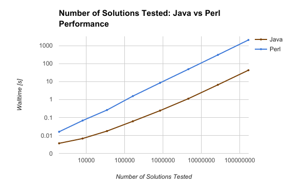
When the wall time for Java and Perl are plotted against the number of solutions tested, an interesting trend emerges: the two scale the same way, with a fixed vertical offset.

Graph of walltime versus number of solutions tested

While this is proving what we already knew, that a compiled language beats a scripted language every time, it also provides proof Perl can scale as well as Java - it just takes significantly more overhead and time per statement.

Why Java Beat Perl

Compiled languages are turned into bytecode and pre-optimized for the processor.

Perl is a scripted and interpreted language, like Python, evaluated piece by piece.

So, we didn't learn anything surprising. But we did find an interesting result - Perl can scale as well as Java in its implementation of the N queens recursive backtracking algorithm.

Sources

  1. "Execution in the Kingdom of Nouns". Steve Yegge. March 2006. Accessed 18 March 2017. <https://web.archive.org/web/20170320081755/https://steve-yegge.blogspot.com/2006/03/execution-in-kingdom-of-nouns.html>

  2. "N-Queens Problem". Rosetta Code, GNU Free Documentation License. Edited 6 March 2017. Accessed 21 March 2017. <https://web.archive.org/web/20170320081421/http://rosettacode.org/wiki/N-queens_problem>

  3. "nqueens.pl". Charles Reid. Github Gist, Github Inc. Edited 20 March 2017. Accessed 20 March 2017. <https://gist.github.com/charlesreid1/4ce97a5f896ff1c89855a5d038d51535>

  4. "NQueens.java". Charles Reid. Github Gist, Github Inc. Edited 20 March 2017. Accessed 20 March 2017. <https://gist.github.com/charlesreid1/7b8d7b9dffb7b3090039849d72c5fff5>

  5. "Devel::NYTProf". Adam Kaplan, Tim Bunce. Copyright 2008-2016, Tim Bunce. Published 4 March 2008. Accessed 20 March 2017. <https://web.archive.org/web/20170320081508/http://search.cpan.org/~timb/Devel-NYTProf-6.04/lib/Devel/NYTProf.pm>

  6. "Perl/Profiling". Charles Reid. Edited 20 March 2017. Accessed 20 March 2017. <https://web.archive.org/web/20170320081532/https://charlesreid1.com/wiki/Perl/Profiling>

  7. "Java/Profiling". Charles Reid. Edited 20 March 2017. Accessed 20 March 2017. <https://web.archive.org/web/20170320081535/https://charlesreid1.com/wiki/Java/Profiling>

  8. "JIP - The Java Interactive Profiler." Andrew Wilcox. Published 30 April 2010. Accessed 20 March 2017. <https://web.archive.org/web/20170320081538/http://jiprof.sourceforge.net/>

  9. "HPROF". Oracle Corporation. Copyright 1993, 2016. Published 2016. Accessed 20 March 2017. <https://web.archive.org/web/20170320081540/https://docs.oracle.com/javase/7/docs/technotes/samples/hprof.html>

Tags:    java    perl    algorithms    recursion    n-queens   

March 2022

How to Read Ulysses

July 2020

Applied Gitflow

September 2019

Mocking AWS in Unit Tests

May 2018

Current Projects