This is Part 3 of a 4-part blog post on the mathematics of the 4x4 Rubik's Cube, its relation to algorithms, and some curious properties of Rubik's Cubes.
See Part 1 of this blog post here: Part 1: Representations
See Part 2 of this blog post here: Part 2: Permutations
You are currently reading Part 3 of this blog post: Part 3: Factoring Permutations
See Part 4 of this blog post here: Part 4: Sequence Order
Table of Contents
Introduction
So far we have been discussing representations of the Rubik's Cube, with the ultimate intention of investigating some of its properties.
In this post, we define and explore the properties we are interested in studying.
Cycles
(Definition of cycle)
We use the two-line notation introduced in the last blog post, so a permutation of a 5-tuple might look like this:
In this permutation, we see that \(a\) and \(b\) swap places, and \(c\), \(d\), and \(e\) exchange places as well. These two groups form two cycles.
Think of the cycles as the particular way that pieces of the permutation are exchanged with one another.
Sequences
We are interested in studying the properties of the cube, but in particular we are interested in the properties of move sequences applied to the cube.
There are 36 possible moves on a cube, and a series of moves applied in a particular order defines a sequence. The 36 possible rotations were given in the prior blog post and cover clockwise and counterclockwise rotations of each of the six faces - either the first layer, the second layer, or both of the first two layers.
These moves are denoted with six letters (UDLRFB) for the upper, downward, left, right, front, and back face of the cube, respectively.
Moves indicated should be clockwise unless they contain an apostrophe
character ', which indicates counterclockwise rotation.
A capital letter indicates a rotation of the first layer only
(e.g., U indicates a clockwise rotation of the first layer of
the upper face).
A lowercase letter indicates a roration of the first and second layers
(e.g., r indicates a clockwise rotation of the top two layers of
the right face).
A 2 before the letter indicates that the second layer should be rotated
(e.g., 2F indicates a clockwise rotation of the second layer of the
front face).
Each move sequence can be translated into a tuple representation (see Part 1 blog post). Once we have the tuple representation of a permutation, we can do several things, beginning with finding the cycles that compose the moves of the sequence.
Order
The quantity we are truly interested in is the order of a given cycle.
The order of a sequence of moves is the number of times that sequence must be applied to the cube to get the cube to return back to its original state. A more convenient way to think about it is, if you applied a move sequence to a solved cube, how many times would you have to apply it until you reached a solved cube again?
We begin with the move sequence, which applies a particular permutation to the cube, exchanging particular pieces in a particular order. We want to obtain a tuple representation of the permutation that results from a particular sequence of moves.
Once we have the tuple representation of a sequence's permutation, we can factor it into independent cycles using the techniques covered in this blog post.
The factoring a permutation into cycles will yield the order; the order is the least common multiple of the lengths of eacch cycle that is a factor.
Using this, we can investigate the properties of the order of different move sequences.
Intercalation Product
In Part 2 of this blog post, we discussed the tuple representation of a permutation; for example, one permutation \(\pi\) of an \(n\)-tuple might be written:
The top row consists of the elements in the tuple in sorted order; the second row consists of elements of the tuple corresponding to that permutation.
In the discussion that follows we'll keep it general, and talk about multisets - the case in which the top row has multiple occurrences of different items.
For the following discussion, we will suppose two permutations \(\alpha\) and \(\beta\) composed of four objects \(\{a, b, c, d,\}\), each occurring multiple times:
Definition
Now we define the intercalation product \(\alpha \top \beta\) of these permutations as the elements of each permutation organized in an interleaved way - each element of \(\alpha\) and \(\beta\) are grouped by the letter that appears on the top row, and within those groups they are ordered as they appear in \(\alpha\), then as they appear in \(\beta\).
For our example, the intercalation product is the following combination of \(\alpha\) and \(\beta\):
This is basically an interleaving operation. All top-bottom pairs with \(a\) at the top are grouped together - and within the group, everyone from \(\alpha\) comes first, everyone from \(\beta\) comes second.
The first two \(a\) items in \(\alpha \top \beta\) come from \(\alpha\), the third \(a\) item comes from \(\beta\).
Side Note: Why Define an Intercalation Product?
You may be wondering what the intercalation product has to do with Rubik's Cubes or finding the order of a sequence. It turns out that the intercalation product will allow us to establish a system of permutation algebra, define certain operations and properties of permutations, and use these to factor permutations into independent groups of faces being exchanged.
Properties
We can state some properties of the intercalation algebra already:
If \(\alpha \top \pi = \beta \top \pi\) or \(\pi \top \alpha = \pi \top \beta\), this implies \(\alpha = \beta\).
An identity element exists such that \(\epsilon \top \alpha = \alpha \top \epsilon = \alpha\).
The commutative property for the intercalation product (whether \(\alpha\) and \(\beta\) can be exchanged in expressions) only holds if \(\alpha\) and \(\beta\) are independent of each other (if they permute different elements). If this condition holds, then \(\alpha \top \beta = \beta \top \alpha\).
This property does not hold in general.
(An example of permutations that would be independent on the Rubik's Cube would be the moves U and D. These each rotate a different group of faces.)
Factoring Permutations Using Knuth's Theorem A
Volume 3 of Donald Knuth's The Art of Computer Programming gives the following theorem on page 26, which gives a very useful property of intercalation products:
Theorem A. Let the elements of the multiset \(M\) be linearly ordered by the relation "<". Every permutation \(\pi\) of \(M\) has a unique representation as the intercalation
where
and
Significance of Factors
Theorem A is central to our goal of studying move sequences (and computing their order). To understand why, consider the factors that result from Theorem A, and what they mean in the specific example of a Rubik's Cube.
In a regular n-tuple, the factors represent groups of items in the tuple that are being exchanged. A tuple that factors into the intercalation of many very small tuples means the permutation mostly consists of swapping pairs or triplets of things. A tuple that factors into the intercalation of two large tuples means, all of the things are divided into two groups, and within that group, everybody is mixed in with everybody else.
On a Rubik's Cube, the tuple consists of faces being moved, so a permutation's factors indicate how many faces are being swapped. The size of each group of faces gives some indication as to how long it takes for the cube to "sync up" with its original state if the permutation is repeatedly applied; a permutation with fewer large factors will take longer than a permutation with many small factors.
For example, suppose a move sequence permutes three corner pieces on a cube each time it is applied. Then if we write the two-line tuple corresponding to that permutation, and we factor it into the intercalation product of several tuples, several factors of the permutation will have a length of three, and will contain the set of three faces being exchanged.
On the other hand, if a move sequence permutes six corner pieces on a cube each time it is applied, some of the factors will be groups of six faces being exchanged when the sequence is applied.
Thus, the (sizes of the) factors of a permutation determine the order of the permutation.
How to Factor Permutations
To factor a permutation, we perform the opposite of the intercalation product. Now supppose we wish to factor the permutation:
into the intercalation of multiple independent, disjoint cycles,
We can extract each factor one at a time using the following algorithm.
Start by assuming the first factor \(\alpha\) contains the first symbol \(a\) in its top row.
(It turns out this assumption can't be false - if there is an \(a\) in the top row of \(\pi\) then there is an \(a\) in the top row of at least one factor. We're simply going to pull out those factors with this assumption.)
Given this assumption, we know \(\alpha\) must map \(a\) to the same letter as the final permutation maps \(a\) to, in the very first column of \(\pi\). The first column of \(\pi\) is \(( a d )\) (a on top, d on bottom). That means that if our assumption holds, if \(\alpha\) contains \(a\), then it must permute all \(a\)'s into \(d\)'s and thus \(\alpha\) should contain the same column \((a d )\).
Now suppose that \(\alpha\) contains \(d\), which it must if our prior step is true. (\(\alpha\) cannot turn \(a\) into \(d\) if it does not have a \(d\)!). We find the leftmost \(d\) on the top line, and see that it maps to the symbol \(d\), due to the column \(( d d )\) (d on top, d on bottom). Thus, \(\alpha\) should also contain the column \(( d d )\).
We keep going. Suppose that \(\alpha\) contains another \(d\), as a consequence of the prior step. Since we already used the first d column in \(\pi\), we use the next column, \(( d b )\) Thus, \(\alpha\) should also contain the column \(( d b )\), and we use the outcome \(b\) as the starting point for the next step.
The process stops as soon as the starting point for the next step is the letter we began with, \(a\). That's because, at that point, we've formed a "closed loop" of pieces that permute with one another. That closed loop forms the first intercalation factor of the permutation \(\pi\).
If we keep repeating the process described, we eventually wind up with \(\alpha\):
Side Note: Why Does This Work?
Let's pause for a moment and see what's happening. What we're doing is following a thread between the top and bottom rows of the permutation; this thread tells us how elements are being moved around to create permutations.
(A simpler but easier way to see this is by comparing two permutations of \((1 2 3 4 5 6)\): consider the permutation \((2 1 3 4 6 5)\), versus the permutation \((2 4 5 6 1 3)\). The first permutation swaps positions 0 and 1, and positions 4 and 5, independently; the second permutation mixes all positions together.)
We are assembling \(\alpha\) piece by piece, by pulling out pairs from the top and bottom row of \(\pi\) and putting them into \(\alpha\). At some point we will come back to the starting point, the symbol \(a\), and we will be finished finding the first factor \(\alpha\), which is a disjoint cycle.
By starting from the top row and following where it leads in the bottom row, and continuing until we return to the original starting element in the top row, we can carve up the permutation into groups of pieces exchanged with one another and not with any other pieces, or groups of pieces that don't move.
How to Factor Permutations (Cont'd)
Recall that our goal was to factor the permutation \(\pi\) into the intercalation of multiple independent and disjoint cycles, \(\pi = \alpha \top \beta \top \dots \top \gamma\). We gave a procedure to extract factors and used it to extract the first factor, \(\alpha\).
However, this is not the end of the factoring process: there are still several elements of \(\pi\) that have not been used to form \(\alpha\), and those remaining elements themselves form a permutation that can be factored.
We begin with the original permutation \(\pi\):
When we pull out the first factor \(\alpha\), we get:
When we pull out the second factor \(\beta\), we get:
The third factor can be pulled out as well, which leaves the last factor, a single column \(( d d )\) by itself, indicating an element that is not moved by the permutation.
Thus the permutation \(\pi\) can be expressed as the intercalation of four independent cycles.
This procedure illustrates Knuth's Theorem A.
(Note: had we initially assumed \(\alpha\) contained \(b\) instead of \(a\), we would end up starting by pulling out a different factor, but we would ultimately end up with the same set of four factors.)
To relate this back to the Rubik's Cube, we can start with a sequence
of interest, like U R D D B, and write the tuple representing the
outcome of this sequence when it is applied to the cube. In this way
we represent a move sequence as a tuple or as a permutation.
Next, we factor this permutation the way we factored \(\pi\), into the intercalation product of independent cycles. These are groups of pieces being swapped each time the cycle is applied.
Now if one factor is of length 4 (group of 4 faces being permuted), one factor is of length 3, and one factor is of length 20, then the number of times the sequence must be applied before the cube will come back to its original, solved state is \(LCM(3,4,20) = 60\).
Algorithm A
Algorithm A is an algorithm written to perform the factoring process described above.
We started with the two-row representation above, so our function will start with the top and bottom rows of the two-row representation.
The procedure started with the first entry of the top row, and got the corresponding entry of the bottom row. It then moved to the index of that item on the top row, and got the coresponding entry of the bottom row, and so on, assembling the components of the permutation by stepping through each.
In code, this will require us to switch between items in a list, and the indices of occurrencs of items in the list. Fortunately, this is an easy and common operation.
Following is the pseudocode, then the Python code, to implement Algorithm A on the two-row representation of a tuple.
Pseudocode
Our function takes two arguments: the top and bottom rows of the two-row representation of this permutation.
define function factor_permutations( top row, bottom row )

    create bit vector to mark columns as factored or not

    initialize list of factors

    initialize pointer to active location

    initialize starting index

    while there are still zeros in the bit vector:

        initialize this factor

        run until break reached:

            set bit vector at active location to 1

            get active location entries on top row (leader) and bottom row (follower)

            get next active location (index of follower in top row)

            break if next active location out of bounds

            break if next active location is starting element

            append follower to this factor

        add starting element to end of factor

        add factor to list of factors

        set next start index to index of first 0 in bit vector

    return factors
Python Code
(Code for Algorithm A)
def factor_permutation(perm_top,perm_bot):
    """
    Factor a permutation into its lowest terms
    """
    MAX = 96
    # Need a way to also mark them as used... bit vector
    used_vector = [0,]*len(perm_top)

    i = 0
    start = perm_top[0]
    used_vector[0] = 1

    factors = []

    # If we still have values to pick out:
    while(0 in used_vector):

        factor = []

        while(True):
            used_vector[i] = 1
            leader = perm_top[i]
            follower = perm_bot[i]

            i = perm_top.index(follower)
            while(used_vector[i]==1):
                i += 1
                if(i>=MAX):
                    break

            if(i>=MAX):
                break
            elif(follower==start):
                break
            else:
                factor.append(follower)

        # add start to end
        factor.append(start)

        factors.append(factor)
        try:
            i = used_vector.index(0)
            start = perm_top[i]
        except ValueError:
            break

    factorsize = set()
    check = 0
    for factor in factors:
        factorsize.add(len(factor))
        check += len(factor)
    return factors
Preview of Part 4
We concluded with an algorithm that will be central to our task of computing the order of a Rubik's Cube move sequence.
In the next post, we'll apply our method of representing Rubik's Cubes using the two-line tuple notation, and use the factoring algorithm above, which will allow us to factor Rubik's Cube permutations into their corresponding intercalation products.
From there, we can count the size of each intercalation product, and the least common multiple of the sizes gives the order of the permutation.
References
-
"Rubik's Cube". Charlesreid1.com wiki, Charles Reid. Edited 20 January 2017. Accessed 20 January 2017. <https://charlesreid1.com/wiki/Rubiks_Cube>
-
"Rubik's Revenge". Charlesreid1.com wiki, Charles Reid. Edited 20 January 2017. Accessed 20 January 2017. <https://charlesreid1.com/wiki/Rubiks_Revenge>
-
"Rubik's Cube/Tuple". Charlesreid1.com wiki, Charles Reid. Edited 20 January 2017. Accessed 20 January 2017. <https://charlesreid1.com/wiki/Rubiks_Cube/Tuple>
-
"Rubik's Cube/Permutations". Charlesreid1.com wiki, Charles Reid. Edited 20 January 2017. Accessed 20 January 2017. <https://charlesreid1.com/wiki/Rubiks_Cube/Permutations>
-
"Github - dwalton76/rubiks-cube-NxNxN-solver". dwalton76, Github Repository, Github Inc. Accessed 11 January 2017. <https://github.com/dwalton76/rubiks-cube-NxNxN-solver>
-
"Rubik's Cube NxNxN Solver". Git repository, git.charlesreid1.com. Charles Reid. Updated 20 January 2017. <https://git.charlesreid1.com/charlesreid1/rubiks-cube-nnn-solver>
-
"Rubiks Cube Cycles". Git repository, git.charlesreid1.com. Charles Reid. Updated 20 January 2017. <https://git.charlesreid1.com/charlesreid1/rubiks-cube-cycles>
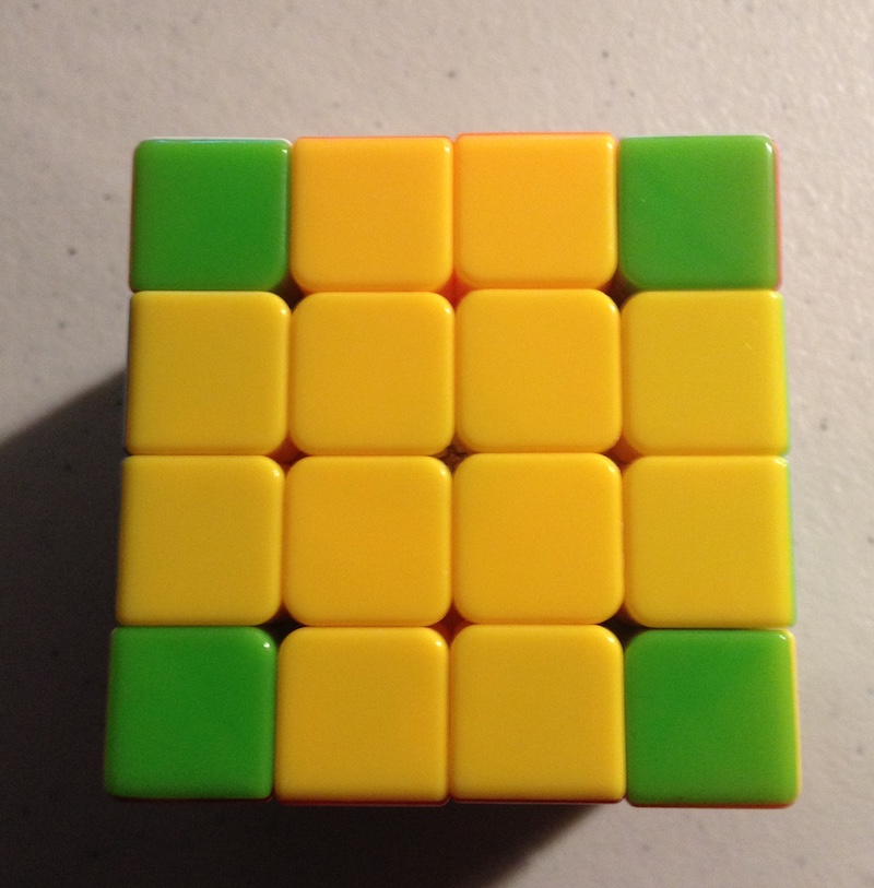 Figure 1: Corner pieces are green.
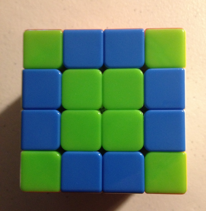 Figure 2: Double edge pieces are blue.
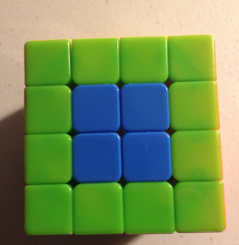 Figure 3: Center pieces are blue.
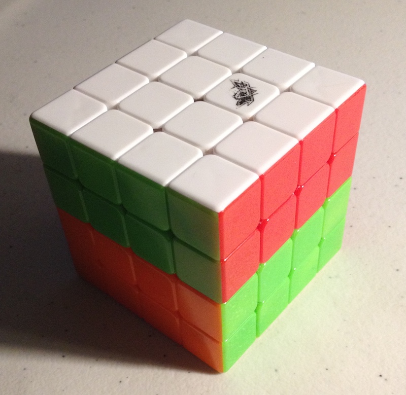 Figure 4: Cube state after move
 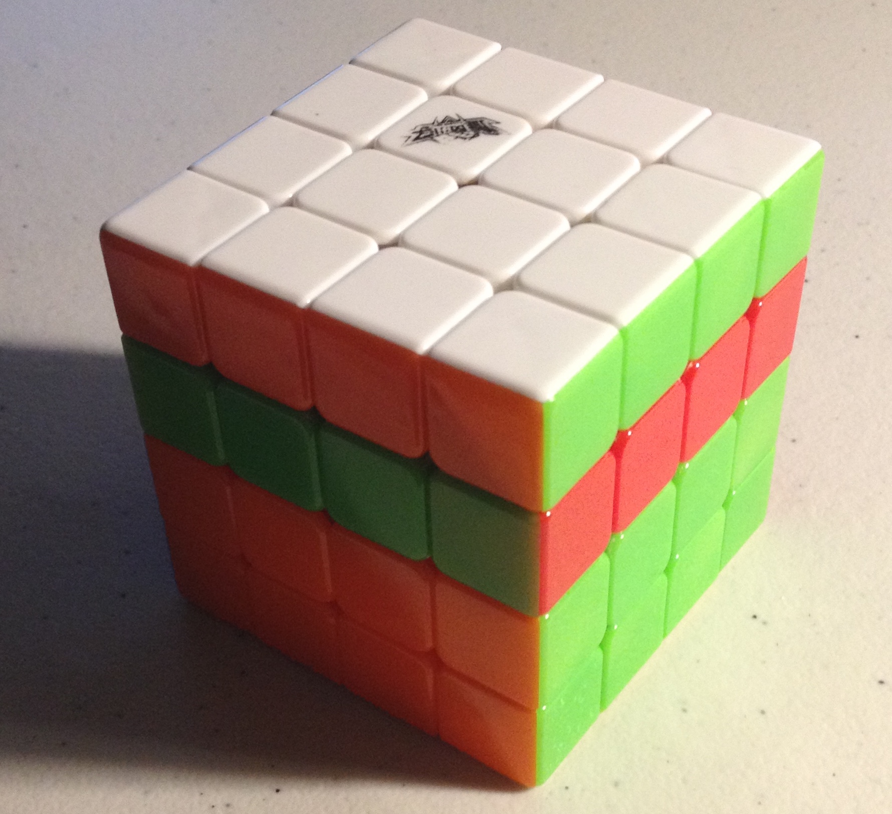 Figure 5: Cube state after move